Data 145 Study Guide — Lectures 14

Comprehensive Study Guide — Lectures 14 through 15 · Spring 2026
Instructors: Ani Adhikari, William Fithian

Bridge: Lecture 13 to Lecture 14

By the end of Lecture 13, the course already has the full testing language: null/alternative, Type I and II error, level, power, NP lemma, and MLR/UMP logic. That part of the course solves an optimization problem: among all tests with controlled Type I error, which rejection rule is strongest against the alternative?

Lecture 13 solves: "what rejection region is best?"
Lecture 14 asks the next natural question: "once we have a test, how should we summarize the evidence in one dataset?"

In practice, a binary reject/do-not-reject answer is too thin. We usually want two richer outputs: a scalar evidence summary telling us how extreme the data are under the null, and a set-valued uncertainty summary telling us which parameter values still look plausible.

This is why Lecture 14 does not replace hypothesis testing; it asks what testing output should look like after the rejection rule has already been designed. P-values and confidence regions are the reporting layer built on top of the Lecture 12-13 testing framework.

Lecture 14: p-values, Confidence Regions, and Test-CI Duality

14.1 p-values formalized

If a test rejects for large values of a statistic $T(X)$, then for a simple null: $$p(x) = P_{H_0}(T(X) \ge T(x)).$$ For a composite null $H_0: \theta \in \Theta_0$: $$p(x) = \sup_{\theta\in\Theta_0} P_\theta(T(X) \ge T(x)).$$

For all valid p-values under the null: $$P_\theta\bigl(p(X)\le\alpha\bigr) \le \alpha, \qquad \theta\in\Theta_0.$$ So rejecting when $p\le\alpha$ always gives a valid level-$\alpha$ test.

A p-value is not $P(H_0\mid\text{data})$.
It is a tail probability of data extremeness assuming $H_0$ is true.

A p-value is not an intrinsic property of the dataset alone. It depends on the chosen test statistic $T(X)$, because $T$ determines what it means for data to be "more extreme" than what was observed.

14.2 Why p-values and confidence intervals can disagree with intuition

Two binomial scenarios from class:

Scenario	n	Heads	$\hat p$	Two-sided p-value for $H_0:p=0.5$	95% CI (normal approx)
A	50	29	0.58	0.3222	[0.443, 0.717]
B	5000	2600	0.52	0.0049	[0.506, 0.534]

Scenario A has a larger observed departure from 0.5 but weak evidence because the sample is small. Scenario B has a tiny departure but strong evidence because precision is high.

14.3 Confidence regions

A $(1-\alpha)$ confidence region for $g(\theta)$ is a random set $C(X)$ such that $$P_\theta\bigl(C(X)\ni g(\theta)\bigr) \ge 1-\alpha \quad \text{for all }\theta.$$

The random object is the interval/region $C(X)$; the true parameter value is fixed. So the 95% statement is about the procedure over repeated samples, not a posterior probability for one realized interval.

14.4 Test-CI duality (the central structural idea)

If $\phi(X;a)$ is a level-$\alpha$ test of $H_0:g(\theta)=a$, then $$C(X)=\{a:\phi(X;a)<1\}$$ is a valid $(1-\alpha)$ confidence region.

Conversely, if $C(X)$ is a valid $(1-\alpha)$ confidence region, then $$\phi(x;a)=\mathbf{1}\{a\notin C(x)\}$$ is a valid level-$\alpha$ test.

A confidence interval is exactly the set of null values that the data do not reject at level $\alpha$.

14.5 What to carry forward

Lecture 14 is mostly structural, not yet constructive. It explains how p-values, tests, and confidence sets are supposed to fit together, but it does not yet tell us which test family to use in a parametric model.

So the next question is practical: with likelihoods, scores, Fisher information, and MLE asymptotics already available from Lectures 3-5, what concrete tests should we actually build and invert?

Bridge: Lecture 14 to Lecture 15

Lecture 14 gives a recipe: for each candidate null value, test it at level $\alpha$, then collect the values not rejected. That recipe is only useful once we know how to manufacture a good test for every possible null value.

Lecture 14 says: confidence regions come from inverting tests.
Lecture 15 says: in parametric models, the local shape of the log-likelihood gives three canonical asymptotic tests to invert.

This bridge directly reuses Lectures 3-5: log-likelihood, score, Fisher information, and MLE asymptotics. The same local quadratic approximation that explained why the MLE is asymptotically normal will now explain why Wald, Score, and GLRT are all valid and closely related.

Lecture 15: Asymptotic Tests (Wald, Score, GLRT)

15.1 Setup recap from earlier lectures

For i.i.d. $X_1,\ldots,X_n\sim f_\theta$: $$\ell_n(\theta)=\sum_{i=1}^n\log f_\theta(X_i),\quad S_n(\theta)=\ell_n'(\theta),\quad I(\theta)=\Var_\theta(\ell_1'(\theta;X_i)).$$ $$\sqrt n(\hat\theta_n-\theta_0)\xrightarrow{d}N\!\left(0,\frac{1}{I(\theta_0)}\right),\qquad \frac{S_n(\theta_0)}{\sqrt{nI(\theta_0)}}\xrightarrow{d}N(0,1).$$

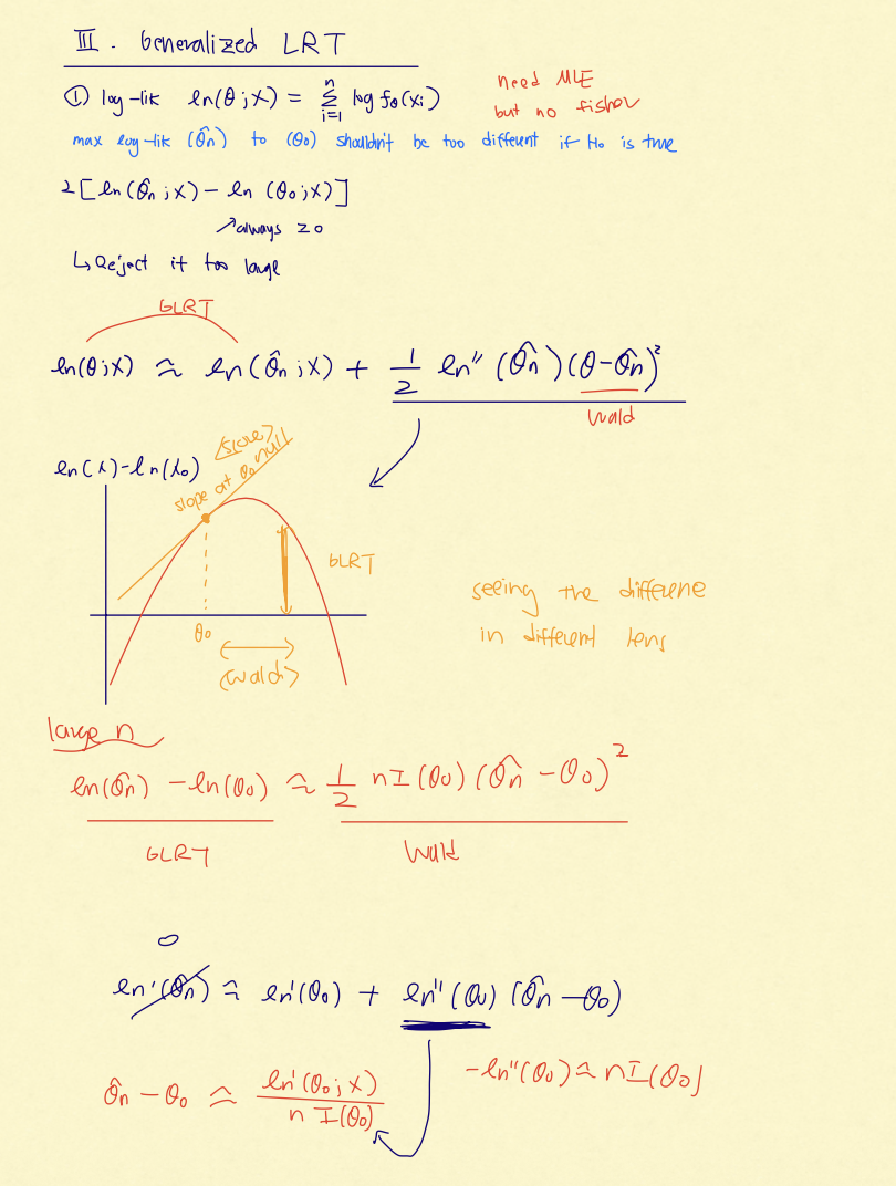
Near $\hat\theta_n$, the log-likelihood is approximately quadratic. Wald, Score, and GLRT are three ways to measure different geometric aspects of this same local shape.

This is the key reuse of earlier material. In Lectures 4-5, the quadratic approximation around the truth produced the asymptotic distribution of the MLE. In Lecture 15, that same parabola is read in three different ways: how far the null is from the peak, how steep the likelihood is at the null, and how much log-likelihood is lost by forcing the null to hold.

15.2 Wald test

$$W=\frac{\hat\theta_n-\theta_0}{\widehat{\text{SE}}(\hat\theta_n)}.$$ Reject for large $|W|$ in two-sided testing.

Wald is convenient but can be sensitive to parameterization and can yield poor finite-sample behavior near boundaries.

15.3 Score test

$$Z=\frac{\ell_n'(\theta_0)}{\sqrt{nI(\theta_0)}}.$$ Reject for large $|Z|$ (two-sided).

Score test advantages:

Does not require computing the MLE
Evaluates directly at the null
Invariant to smooth reparameterization

15.4 Generalized likelihood ratio test (GLRT)

The likelihood ratio test from Lectures 12-13 compared two fixed parameter values. GLRT is the composite-hypothesis version: compare the best likelihood allowed by the full model to the best likelihood allowed by the null model.

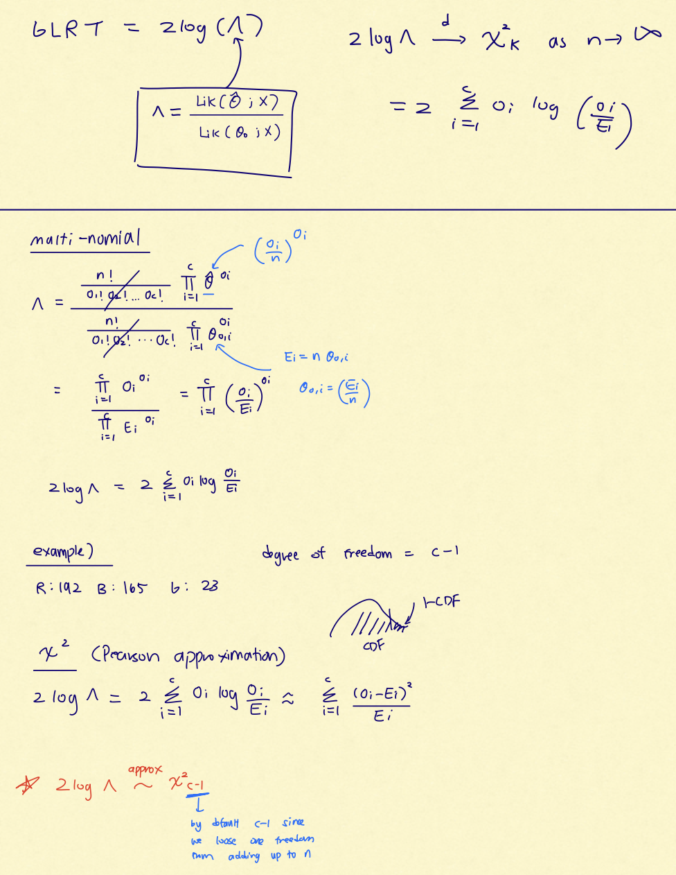
For i.i.d. data, write $$\ell_n(\theta)=\sum_{i=1}^n \log f_\theta(X_i).$$ Let $\hat\theta_n$ be the unrestricted MLE, and let $\hat\theta_{0,n}$ be the MLE constrained to $H_0$. Using the full-over-null convention, $$\text{LR}_n(\mathbf{X})=\frac{L_n(\hat\theta_n)}{L_n(\hat\theta_{0,n})},\qquad 2\log\text{LR}_n(\mathbf{X})=2\{\ell_n(\hat\theta_n)-\ell_n(\hat\theta_{0,n})\}.$$

GLRT measures the vertical drop from the best possible log-likelihood to the best null-constrained log-likelihood. The unrestricted fit can only improve the likelihood, so $2\log\text{LR}_n(\mathbf{X})\ge 0$. If $H_0$ is true, the two fits should not be very different; reject for large $2\log\text{LR}_n(\mathbf{X})$.

Why a chi-squared limit appears

For a one-dimensional null such as $H_0:\theta=\theta_0$, the null-constrained MLE is just $\theta_0$. Since $\ell_n'(\hat\theta_n)=0$, a Taylor expansion around $\hat\theta_n$ gives

$$\ell_n(\theta_0)\approx \ell_n(\hat\theta_n)+\frac{1}{2}\ell_n''(\hat\theta_n)(\theta_0-\hat\theta_n)^2.$$

$$2\{\ell_n(\hat\theta_n)-\ell_n(\theta_0)\}\approx -\ell_n''(\hat\theta_n)(\hat\theta_n-\theta_0)^2.$$

This is why GLRT is secretly measuring the same local quantity as Wald: distance from $\theta_0$ to $\hat\theta_n$, scaled by curvature. Under $H_0$, the scaled distance behaves like a squared standard normal, so the statistic converges to $\chi^2_1$.

More generally, if the null imposes $k$ restrictions, Wilks' theorem gives $$2\log\text{LR}_n(\mathbf{X})\xrightarrow{d}\chi^2_k.$$

Multinomial goodness-of-fit connection

For multinomial counts, GLRT becomes especially concrete. Suppose there are $c$ categories, observed counts $O_i$, and null expected counts $E_i=n\theta_{0,i}$. The unrestricted MLE is $\hat\theta_i=O_i/n$, so

$$2\log\text{LR}(\mathbf{O})=2\sum_{i=1}^c O_i\log\left(\frac{O_i}{E_i}\right).$$

Under the multinomial null, $$2\log\text{LR}(\mathbf{O})\xrightarrow{d}\chi^2_{c-1}.$$ The degree of freedom is $c-1$ because the category probabilities must sum to 1, so only $c-1$ components are free.

Pearson's chi-squared statistic is the local quadratic approximation to the likelihood-ratio statistic: $$2\sum_{i=1}^c O_i\log\left(\frac{O_i}{E_i}\right)\approx \sum_{i=1}^c \frac{(O_i-E_i)^2}{E_i}.$$ So both are checking whether the observed count vector is unusually far from the expected count vector.

15.5 Poisson running example ($n=30$, $\bar X=3.07$)

For $X_i\sim\text{Pois}(\lambda)$, class comparisons give:

Method	95% interval for $\lambda$	Comment
Wald	[2.443, 3.697]	Symmetric around $\bar X$
Score	[2.504, 3.764]	Respects positivity naturally
GLRT	[2.485, 3.740]	Likelihood-based inversion

15.6 Unifying equivalence statement

Locally under $H_0$: $$W^2 \approx Z^2 \approx 2\bigl[\ell_n(\hat\theta_n)-\ell_n(\theta_0)\bigr] \xrightarrow{d} \chi^2_1.$$ So all three tests are asymptotically equivalent; finite-sample differences come from how imperfect the quadratic approximation is.

Normal mean with known variance gives an exactly quadratic log-likelihood, so Wald, Score, and GLRT coincide exactly. Poisson is only approximately quadratic near the MLE, so small finite-sample differences remain.

Big Transition Map

Master Summary & Formula Sheet

Core lecture-14 formulas

Core lecture-15 formulas

Lecture stage	Main question answered	How it connects forward
11 (KS / empirical CDF)	How to test whole-distribution fit	Prepares broader testing language
12–13 (NP, MLR, UMP)	What rejection rule is optimal	Creates the test design framework but not yet the reporting language
14 (p-values, CIs, duality)	How to summarize evidence and plausible parameter values	Turns a family of tests into a family of confidence sets
15 (Wald, Score, GLRT)	How to build practical asymptotic tests from likelihood theory	Specializes the general testing framework using likelihood geometry and sets up later chi-squared/GLRT ideas

Object	Formula	Meaning
Simple-null p-value	$p(x)=P_{H_0}(T(X)\ge T(x))$	Tail extremeness under null
Composite-null p-value	$p(x)=\sup_{\theta\in\Theta_0}P_\theta(T(X)\ge T(x))$	Worst-case null calibration
Super-uniformity	$P_\theta(p\le\alpha)\le\alpha$	Guarantees valid level control
Confidence region	$P_\theta(C(X)\ni g(\theta))\ge 1-\alpha$	Procedure-level coverage
Test->CI inversion	$C(X)=\{a:\phi(X;a)<1\}$	Set of non-rejected null values

Test	Statistic	Reads what geometric feature?
Wald	$W=(\hat\theta-\theta_0)/\widehat{SE}$	Horizontal distance
Score	$Z=\ell_n'(\theta_0)/\sqrt{nI(\theta_0)}$	Slope at null
GLRT	$2[\ell_n(\hat\theta)-\ell_n(\hat\theta_0)]$	Vertical drop from full fit to null fit
Equivalence	$W^2\approx Z^2\approx 2[\ell_n(\hat\theta)-\ell_n(\theta_0)]$	Same local quadratic backbone

Practical guidance:
Use Wald for convenience when MLE is already in hand, Score when null-evaluation and invariance matter, and GLRT when likelihood comparison is the natural primary object.

Common Mistakes to Avoid

1. "$p<0.05$ means the null is probably false."
No. p-value is computed under the null, not a posterior null probability.

2. "$p>0.05$ means no effect."
No. It may reflect low power or poor targeting of alternatives.

3. "A realized 95% CI contains the truth with 95% probability."
No. Frequentist 95% is long-run coverage of the method.

4. "Wald, Score, and GLRT always agree."
Only asymptotically; finite-sample behavior can differ.

5. "Asymptotic normal confidence intervals are always fine."
Near boundaries or under awkward parameterization, Score/GLRT-inverted confidence regions can be safer.

Data 145: Evidence and Uncertainty

Table of Contents