Transformer, Scaling, and Efficiency

This post summarizes my notes for studying background knowledge / summary for scaling and efficiency.

Transformers

Vanilla Transformer has MHA (Multi-Head Attention). The improvements are mainly made by adjusting the dimension of heads.

MQA (Multi-Query Attention) [2019, Noam Shazeer]

“However, when generating from the trained model, the output of the self-attention layer at a particular position affects the token that is generated at the next position, which in turn affects the input to that layer at the next position. This prevents parallel computation.”

But we can still make incremental steps cheaper. It is mainly through removing the H dim.

MHA (Multi-Head Attention) → MQA (Multi-Query Attention), GQA (Grouped Query Attention)

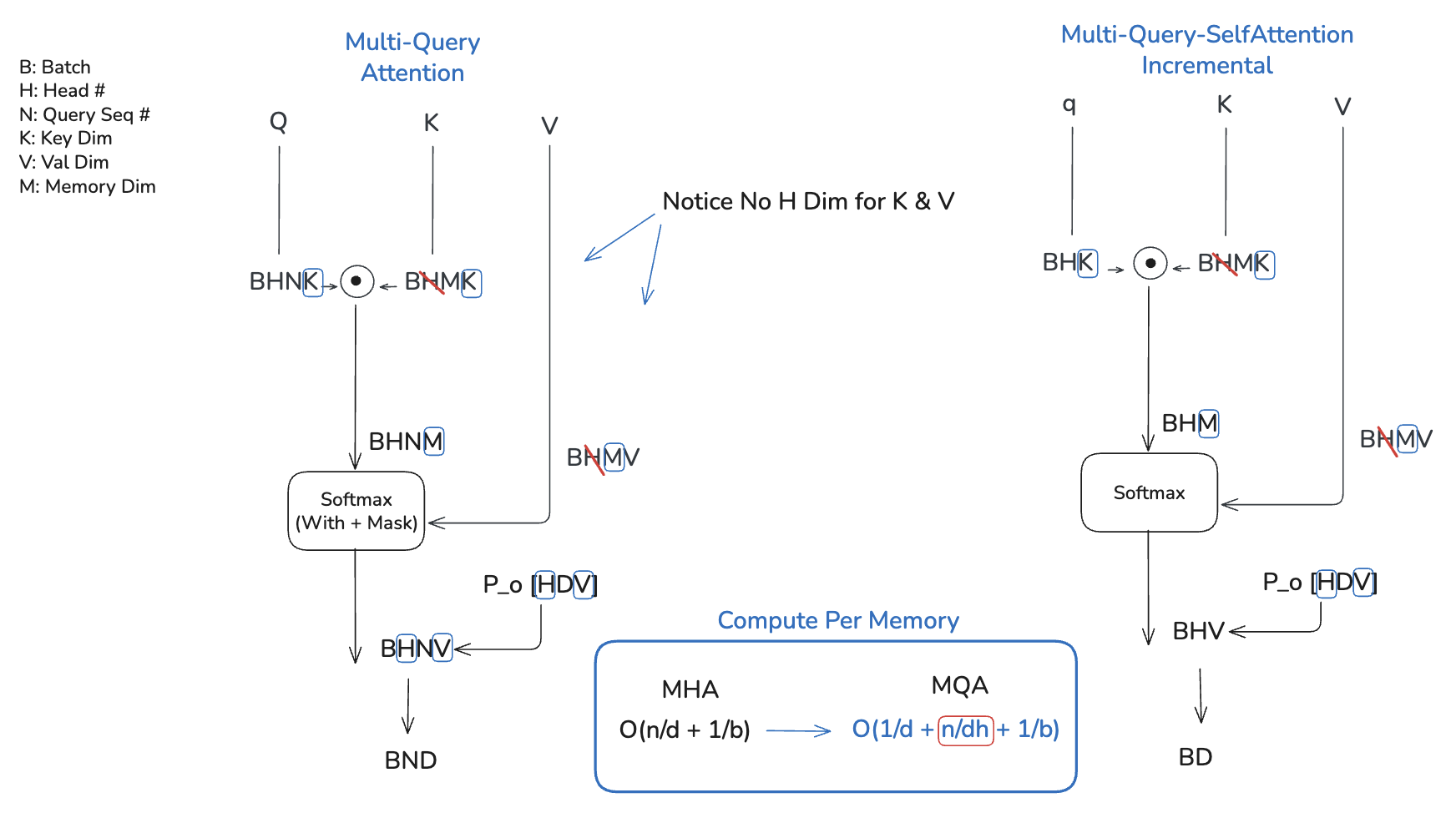
Figure: Multi-Query Attention (MQA) overview.

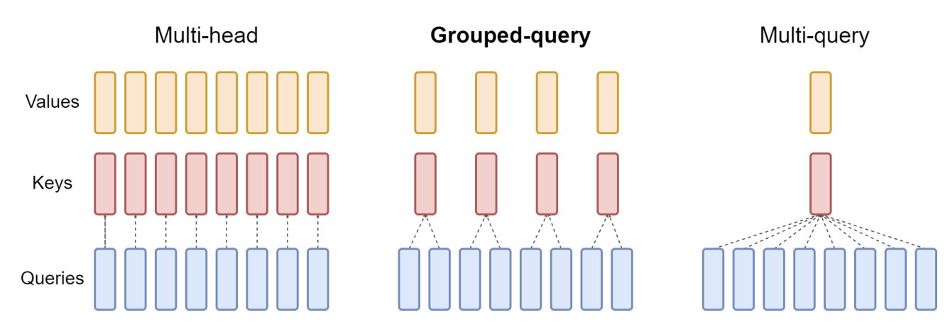
GQA (Grouped Query Attention) [2023, J Ainslie et. al]

“However, multi-query attention (MQA) can lead to quality degradation and training instability, and it may not be feasible to train separate models optimized for quality and inference.”

Uptrain: MHA -> GQA: You can pool and combine the initial ones without having to train from scratch.
GQA: Simply the middle ground between MHA and MQA. Which is why it mentions based on the count it just becomes MHA or MQA.

“Grouped-query attention divides query heads into G groups, each of which shares a single key head and value head. GQA-G refers to grouped-query with G groups. GQA-1, with a single group and therefore single key and value head, is equivalent to MQA, while GQA-H, with groups equal to number of heads, is equivalent to MHA.”

Parallels

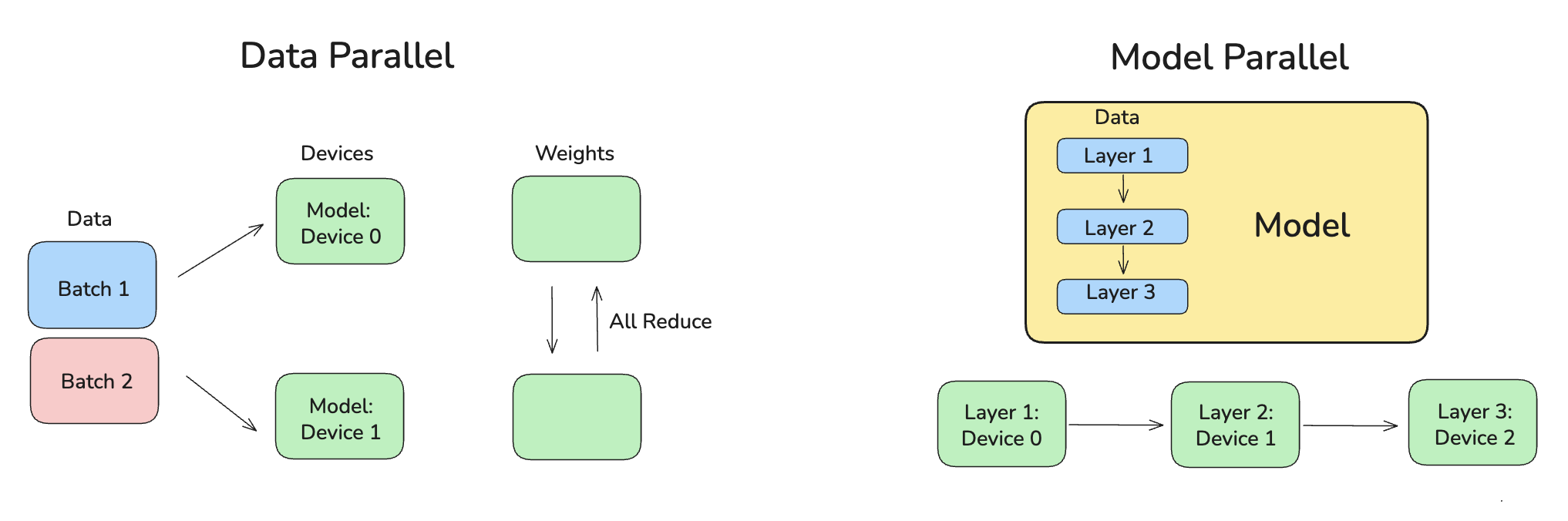
Data Parallel

Each device each has a copy of the model, and gets independent batch of data.

Limitations

HBM capacity: the full model must fit on each device.
Too much communication (e.g., all-reduce)

Model Parallel

The model layers itself is split across different devices. This allows bigger models to be split and fit to devices.

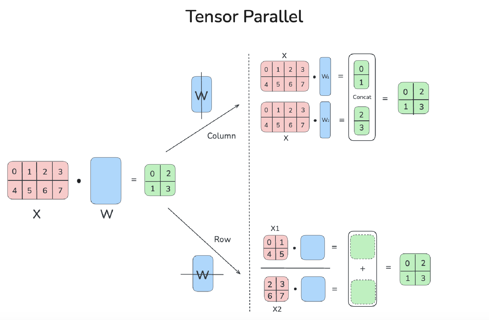
Tensor Parallel

Tensor Computation itself is split across different devices.

Mixture of Experts (MoE): why it shows up in “efficient modeling”

Main idea / Why MoE is “efficient”

MoE uses conditional computation: instead of running the same dense subnetwork for every token, a router (gating network) selects a small number of experts per token. This allows “model capacity to increase without proportional increase in computational cost”.

1) Compute efficiency (FLOPs/token):
You only run a small subset of experts per token (e.g., top-1 or top-2), so you avoid paying dense compute everywhere.

2) Scaling efficiency (quality-per-compute):
For the same FLOPs budget, MoE often buys you a larger effective parameter count.

Core challenges

1) Expert starvation (a.k.a. “shrinking batch”)

If you have many experts, a small batch can’t populate them well.

Let:

(N): total number of experts
(K): number of selected experts per token (top-(k))
(B): local batch size (tokens/examples) per device
(D): number of devices

Expected tokens per expert (very roughly):

tokens_per_expert ≈ (K / N) * B

“This causes a naive MoE implementation to become very inefficient as the number of experts increases. The solution to this shrinking batch problem is to make the original batch size as large as possible. However, batch size tends to be limited by the memory necessary to store activations between the forwards and backwards passes.”

Solution: Data Parallelism + Model Parallelism

With this parallel, we go from first to second (N/K) * B « (N/K) * B * D

2) Communication bottleneck (stationary experts)

Experts are typically stationary on certain devices. Tokens must be dispatched to the expert’s device and then collected back.
If each expert does only a tiny amount of compute, GPUs can become network-bound (waiting on transfers)

Solution: Increase compute-per-byte (arithmetic intensity)
“To maintain computational efficiency, the ratio of an expert’s computation to the size of its input and output must exceed the ratio of computational to network capacity of the computing device.’

The point is not “communication time decreases.”
It’s: if communication is fixed, make the expert compute large enough that communication becomes hidden/overlapped and no longer dominates step time.

“Conveniently, we can increase computational efficiency simply by using a larger hidden layer, or more hidden layers.”

3) Load balancing (avoid routing collapse)

Without constraints, the router might send too many tokens to a few experts.

Common strategies:

Auxiliary balancing losses (e.g., importance / load losses based on coefficient of variation)
Noise on routing logits (e.g., Gaussian noise) to encourage exploration early
Capacity limits per expert (drop/overflow strategies)

Goal: keep usage reasonably spread so all experts train and hardware stays utilized.

(Switch Transformer) Why MoE pairs naturally with Transformers

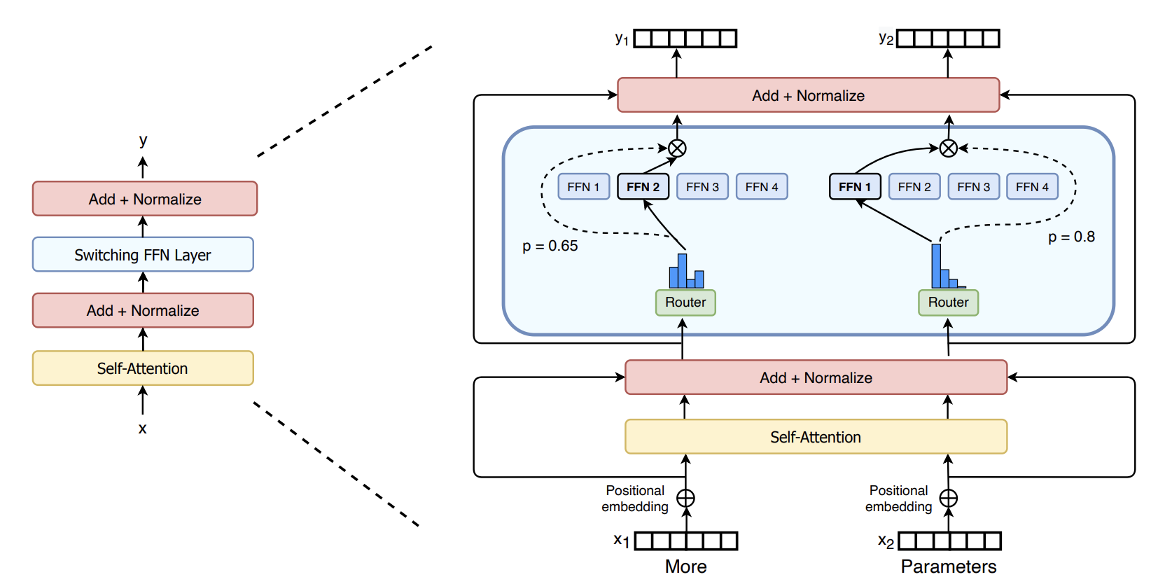
RNN-style model has strong sequential dependencies across timesteps during training that makes “one giant batch over time” harder to exploit. The limitation of the MoE as athor suggested “we wait for the previous layer to finish, we can apply the MoE to all the time steps together as one big batch” If you try to put an MoE inside an RNN (like an LSTM), the “one timestep depends on the output of the MoE at the previous timestep”

In contrast, Transformers enable large, parallel token computation during training (within a sequence and across sequences), which makes it easier to form big token batches for MoE routing.

“we investigate a fourth axis: increase the parameter count while keeping the floating point operations (FLOPs) per example constant” - Switch Transformers [2021]

This is one practical reason MoE is often discussed as “Transformer + sparse FFN”:

keep attention dense (or not—orthogonal choice),
swap dense FFN blocks for MoE / Switch FFN blocks.

KV Cache, Flash Attention, Paged Attention, Sliding Window Attention

Great blog below https://www.omrimallis.com/posts/techniques-for-kv-cache-optimization/

Thoughts

I believe these philosophies are very useful for scientific models, especially as we scale them up. For example, Model parameters for genomic language models are also slowly increasing, and the same ideas should be useful for catching up with this trend.

This naturally raises the question I’m trying to explore next: how alternative generation regimes (e.g., Diffusion Language Models) shift the bottlenecks—memory, communication, and parallelism.

Key references

[2019] Fast Transformer Decoding: One Write-Head is All You Need — Noam Shazeer
[2023] GQA: Training Generalized Multi-Query Transformer Models from Multi-Head Checkpoints — Joshua Ainslie, James Lee-Thorp, Michiel de Jong, Yury Zemlyanskiy, Federico Lebrón, Sumit Sanghai
[2017] Outrageously Large Neural Networks: The Sparsely-Gated Mixture-of-Experts Layer — Shazeer et al.
[2021] Switch Transformers: Scaling to Trillion Parameter Models with Simple and Efficient Sparsity — Fedus et al.
[2022] Sparse Upcycling: Training Mixture-of-Experts from Dense Checkpoints — Komatsuzaki et al.