Explainable AI (XAI) and Model Interpretability (SHAP, Integrated Gradients, and Sparse Autoencoders)

Often we use models to make useful predictions.
But in many settings—especially science and clinical decision making—the more important question becomes:

Q. Why did the model make this prediction?
Q. What evidence is it using, and is that evidence trustworthy?

This post is a future-me-friendly overview of the main interpretability “toolbox.”
I’m not trying to be exhaustive—just to collect the core ideas (and the equations I always end up re-deriving).

I. Motivation: what does “interpretability” even mean?

Interpretability tends to show up in a few recurring “jobs to be done”:

Debugging: locate failure modes and spurious shortcuts
(e.g., train a simple probe/tree on internal embeddings and see where errors cluster)
Scientific insight: suggest mechanisms / hypotheses to test
(e.g., which genes / residues / motifs are driving a model’s decision)
Reducing search space: highlight “where to look” so downstream experiments are cheaper
(in my case: using saliency to narrow design/exploration in photonics)

Two useful mental splits:

Local explanations: why this example got this prediction
Global explanations: what generally drives behavior across a dataset

And another split:

Attribution methods: assign credit to inputs (tokens, pixels, genes, atoms)
Representation methods: understand internal features (what does the model encode?)

II. A tiny taxonomy (toolbox map)

Here are the buckets I generally play around with:

Feature Attribution
- Shapley / SHAP
- Integrated Gradients (IG), saliency variants
Perturbation / Counterfactual-style tests
- occlusion / ablations
- LIME (local surrogate models)
- permutation importance
Representation-level interpretability
- Sparse Autoencoders (SAEs), “dictionary learning” on activations
Process interpretability (systems / agents)
- tool traces, intermediate steps, verifiable logs

III. Feature attribution

Shapley values

Imagine three people (Alice, Bob, Charlie) made profit from running a coffee + donut shop.
Can we say each person contributed equally? Probably not—maybe Alice brings baking skill, Bob is a trained barista, and Charlie handles operations.

So the question becomes:

Q. How do we fairly distribute the profit across contributors?

The Shapley idea (from cooperative game theory) is:
give each contributor their average marginal gain across all possible “join orders.”

Concretely, you can think in terms of “difference made when I add you”:

value(Alice + Bob) − value(Alice)
value(Bob + Charlie) − value(Charlie)
value(Bob) − value(nobody)
…and average over all contexts where Bob could be added.

That “average marginal contribution over all coalitions” is what the equation captures.

A common ML setup:

model: $f(x)$
baseline value: $v(\emptyset)$ (often $\mathbb{E}[f(X)]$ over a background dataset)
value function for a subset $S$:

\[v(S) = \mathbb{E}[f(X)\mid X_S = x_S]\]

Then the Shapley value for feature $i$ is:

\[\phi_i = \sum_{S \subseteq N\setminus\{i\}} \frac{|S|!(|N|-|S|-1)!}{|N|!} \Big(v(S\cup\{i\}) - v(S)\Big)\]

Interpretation: average “gain” when feature $i$ is added, across all possible contexts.

Why this is attractive: it satisfies fairness axioms (symmetry, dummy feature gets 0 credit, etc.), and yields the decomposition:

\[f(x) \approx v(\emptyset) + \sum_{i=1}^d \phi_i\]

(“baseline + contributions = prediction”)

A practical note: SHAP

In practice we rarely compute exact Shapley values (exponential subsets).
SHAP is a family of algorithms that approximate or compute them efficiently for certain model classes (e.g., TreeSHAP for trees).

The subtle part: correlations / “missingness”

Shapley values require a value function $v(S)$: “what does the model predict if I only know features $S$?”
But $f(x)$ expects a full input, so we must define what it means for features $\bar S$ to be “missing.”
That choice is exactly where conditional vs. interventional SHAP differs.

Option A — Conditional (correlation-aware)

\[v_{\text{cond}}(S) = \mathbb{E}[f(X)\mid X_S = x_S]\]

Interpretation: average over the missing features in a way that stays realistic given $x_S$.
If features are correlated, knowing $X_S$ already partially determines $X_{\bar S}$, so adding another correlated feature often gives smaller marginal gain → credit gets shared/diluted.

Option B — Interventional (break correlations)

\[v_{\text{int}}(S) = \mathbb{E}_{X_{\bar S}}[f(x_S, X_{\bar S})]\]

Interpretation: keep $x_S$ fixed, but sample the rest independently from their marginals.
This allows unrealistic combinations when features are correlated, so adding a correlated feature can look more impactful → credit becomes more separated across correlated variables.

Why this matters (quick example)

Two biomarkers $X_1, X_2$ rise together.

Conditional: if $X_1$ is high, the model already expects $X_2$ is high → $X_2$ adds less.
Interventional: $X_2$ is no longer predictable from $X_1$ → $X_2$ can add a lot.

So in correlated scientific/clinical data, your SHAP results can change a lot depending on how you define “missing.”

Practical takeaway

Use conditional if you want explanations “on the data manifold” (often best for science).
Use interventional for “what-if we set this feature” style analysis (not automatically causal).
If possible, run both and treat disagreements as a correlation warning sign.

Example: molecules / atoms

A common workflow in cheminformatics is:

compute feature attributions (often SHAP)
map contributions back onto atoms/bonds to highlight which substructures drive the prediction

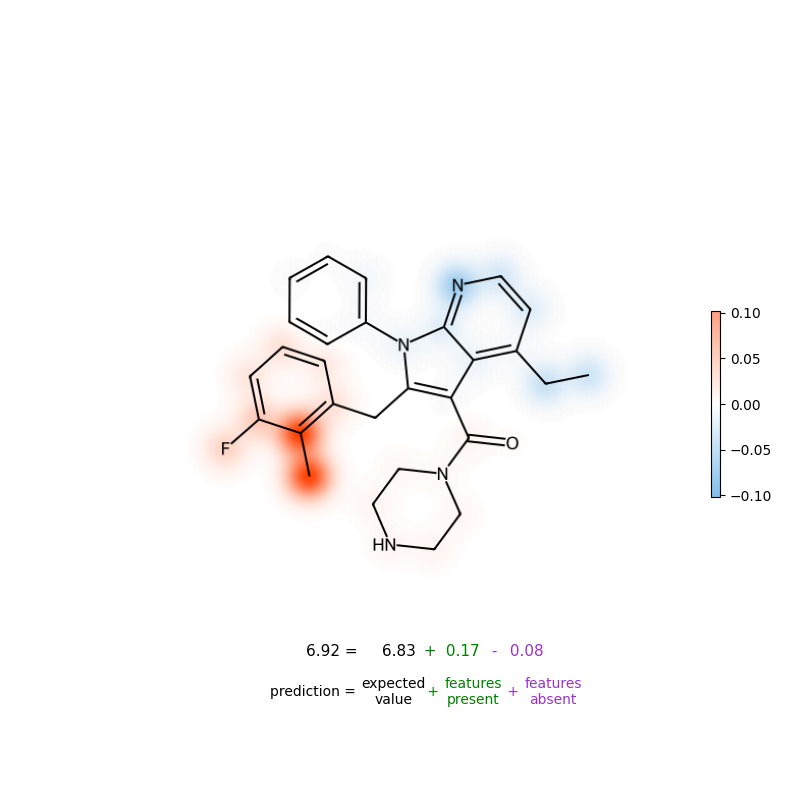
Figure: Atom-level attribution visualization (example).

Integrated Gradients (saliency that “sums to the difference”)

Shapley/SHAP is conceptually clean, but can be heavy and sometimes too coarse when you want a fine-grained saliency map.

Integrated Gradients (IG) answers:

Q. How much did each input dimension contribute, measured via gradients, but in a way that’s less brittle than a single gradient at one point?

Given:

input $x$
baseline $x’$ (e.g., all-zeros image, reference sequence embedding, etc.)
a straight-line path $x(\alpha)=x’ + \alpha(x-x’)$

IG for feature $i$ is:

\[\mathrm{IG}_i(x) = (x_i - x'_i) \int_0^1 \frac{\partial f(x' + \alpha(x-x'))}{\partial x_i} \, d\alpha\]

Key property (completeness):

\[\sum_i \mathrm{IG}_i(x) = f(x) - f(x')\]

So IG gives a clean “baseline + attributions = prediction difference” story.

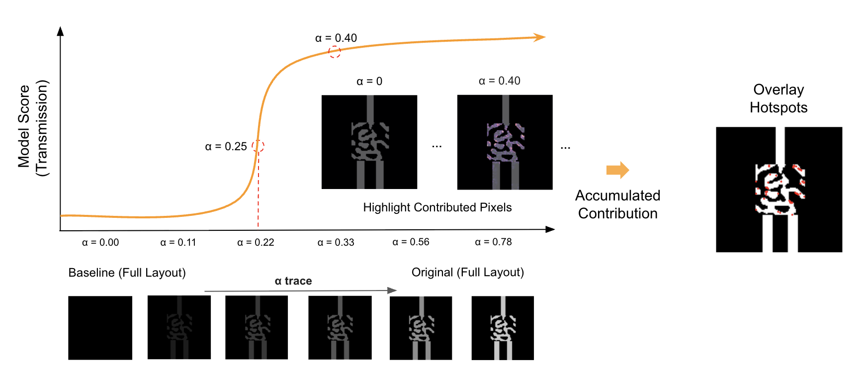
Integrated Gradients alpha trace on a photonics device

Figure: Integrated Gradients visualization from my photonics work (example).

Practical note: for text / discrete tokens

Gradients are defined in continuous space, so for tokens we usually apply IG on:

token embeddings, or
input one-hot relaxed into a differentiable representation

The Core Takeaway before IV.

Shapley/SHAP: “fair credit” averaged over all feature orderings; strong axiomatic story, but can be expensive and sensitive to how you define “missing features.”
Integrated Gradients: path-integrated gradients from a baseline; produces dense saliency maps and satisfies a useful completeness property.
The two biggest foot-guns in practice are: baseline choice and feature correlations.

IV. Perturbation-style interpretability (simple but powerful)

Sometimes the cleanest question is:

Q. If I delete or mutate this feature, does the prediction change?

These methods are often slower (many forward passes), but they’re extremely intuitive and tend to be strong sanity checks.

Occlusion / ablation

Mask a token span / image patch / gene set
Measure $\Delta f = f(x) - f(x_{\text{masked}})$

Permutation importance (more global)

Shuffle a feature across the dataset
Measure performance drop (AUC, accuracy, etc.)

LIME (local surrogate)

LIME builds an interpretable surrogate model around a single point:

sample perturbed versions of $x$
weight them by proximity to $x$
fit a simple model (often linear) to approximate $f$ locally

This is useful when gradients are unreliable or the model is non-differentiable, but it inherits the usual “local linear approximation” limitations.

V. Sparse Autoencoders (representation-level interpretability)

Attribution explains inputs → output.
But it doesn’t tell you what the model internally represents, especially in large models.

This is where SAEs come in:

Q. Can we learn a sparse “dictionary” of features that explains the model’s hidden activations?

Let $a \in \mathbb{R}^m$ be an activation vector from some layer (MLP activations, attention outputs, etc.).
An SAE learns:

encoder: $z = \mathrm{enc}(a)$ (sparse latent)
decoder: $\hat a = W_d z$ (reconstruction)

A common objective is:

\[\min_{\theta} \;\; \|a - \hat a\|_2^2 + \lambda \|z\|_1 \quad \text{where } \hat a = W_d z\]

with an overcomplete latent $z \in \mathbb{R}^k$ (often $k \gg m$), but constrained to be sparse.

…

What you should take away from this post

Interpretability is a toolbox, not a single method.
Attribution (Shapley/SHAP, IG) explains inputs → outputs.
Perturbation tests ask “what changes if I remove/mutate this?”
SAEs shift the question to internal representations and can sometimes enable feature steering.
The most common practical pitfalls are baseline choice and correlations.

Key references

Templeton et al., “Scaling Monosemanticity: Extracting Interpretable Features from Claude 3 Sonnet”, Transformer Circuits Thread, 2024.
Cunningham, Hoagy, et al. “Sparse autoencoders find highly interpretable features in language models.” arXiv:2309.08600 (2023).
Simon, Elana, and James Zou. “InterPLM: discovering interpretable features in protein language models via sparse autoencoders.” Nature Methods (2025).
Sundararajan et al., “Axiomatic Attribution for Deep Networks” (Integrated Gradients), 2017.
Lundberg & Lee, “A Unified Approach to Interpreting Model Predictions” (SHAP), 2017.
https://github.com/basf/MolPipeline