Training a Language Model from Scratch (Part 1: Building Blocks)
This is for future me when I need to review the building blocks of an LM.
While working through CS336 Assignment 1, I kept running into places where I thought I understood the concept, but the implementation details exposed a missing piece. RoPE was not just “add position somehow”; the tokenizer was not the same thing as the embedding layer; cross entropy was not just “take softmax and index the answer”; gradient clipping was not per-parameter clipping.
This post is a cleaned-up version of those notes and aha moments. It is not meant to be a full assignment solution dump. It is the map I want future me to have when I need to reload how the pieces connect: tokenizer, embeddings, RoPE, attention, normalization, feed-forward layers, loss, optimization, and decoding.
Background refresher
Before the implementation details, I want to keep a small shelf of background notes I can come back to. Some of these are notes I created while course staff, and some are materials Sarah Pohland created during the semester. I like them because they connect the Transformer machinery back to a few intuitive ideas: similarity as an inner product, dimensions, attention masks, and training vs inference.
Background notes and handouts
- Main reference: Stanford CS336 Spring 2025
- Discussion Mini Lecture 10: self-attention, inner products, and scaled dot-product attention
- Discussion Walkthrough 10: Q/K/V and scaled dot-product examples
- Discussion Mini Lecture 11: Transformer flow, masking, inference, and KV cache
- Discussion Walkthrough 11: positional encoding and RoPE derivation
- Disc08 Terry notes and Dis09 Terry notes
- CS336 Assignment 1 handout
Attention refresher: what the notes are trying to make intuitive
The attention score is built from an inner product:
\[z_{n,i} = q_n^\top k_i\]The query says what the current token is looking for. The key says what each candidate token exposes. A large dot product means the two vectors are pointing in a similar direction, so the current token should pay more attention to that earlier token.
In matrix form:
\[Q = XW_Q,\quad K = XW_K,\quad V = XW_V\] \[\text{Attention}(Q,K,V) = \text{softmax}_{\text{row}}\left(\frac{QK^\top}{\sqrt{d_k}}\right)V\]The row-wise softmax turns each row of similarity scores into a distribution over which previous tokens to read from. The scale factor $\sqrt{d_k}$ keeps dot products from growing too large as the key/query dimension increases.
For language modeling, the causal mask blocks future positions. During training, we process the whole chunk at once, but position $i$ is only allowed to see positions $\leq i$, matching the information it would have during inference.
The map of the building blocks
raw text <-> token IDs
token ID -> learned vector row
RMSNorm, MHA + RoPE, SwiGLU
hidden row -> vocab logits
cross entropy, AdamW, clipping, schedule
last logits -> next sampled token
"the" -> 391 Names chunks of bytes/text with integer IDs.
391 -> E[391, :] Learns a vector row for each ID.
QK.T -> weights Moves information across positions.
h_i -> logits_i Predicts the next token ID at each position.
I. Tokenizer: byte-level BPE
The tokenizer is not learning semantic vectors. It is deciding how raw text is split into chunks, and mapping each chunk to an integer ID.
The byte-level BPE tokenizer starts with a universal fallback:
| Initial token ID | Token bytes | Meaning |
|---|---|---|
0 | bytes([0]) | byte value 0 |
1 | bytes([1]) | byte value 1 |
... | ... | ... |
255 | bytes([255]) | byte value 255 |
For English, many characters are one byte:
\[\texttt{"t"} \to 116 \to \text{ID }116\]For Korean, one visible character may require multiple UTF-8 bytes:
\[\texttt{"한"} \to [237, 149, 156]\]So initially, "한" might be represented by three byte-level token IDs. If it appears often enough in the training corpus, BPE may learn a merged token for those bytes, letting "한" become one token ID.
237 from "한" is just the fragment b"\xed"; it only decodes properly together with the following bytes. BPE training
BPE training is where the vocabulary grows. The sequence gets more compact, but the vocabulary gets larger.
The high-level loop is:
- Start with the 256 byte tokens, plus special tokens like
<|endoftext|>. - Pre-tokenize raw text into rough chunks.
- Count repeated pre-tokens.
- Convert each pre-token to UTF-8 byte pieces.
- Count adjacent byte/token pairs, weighted by pre-token frequency.
- Merge the most frequent adjacent pair globally.
- Repeat until the target vocab size is reached.
Example:
| Step | Representation | What changes? |
|---|---|---|
| Raw text | "some text" | Original string. |
| Pre-tokenize | ["some", " text"] | Rough chunks, often preserving leading spaces. |
| Count | {" text": 10} | Repeated chunks are stored once with frequency. |
| Bytes | (b" ", b"t", b"e", b"x", b"t"): 10 | Every pre-token becomes byte pieces. |
| Pair counts | (b"t", b"e") += 10 | Adjacent pairs get weighted counts. |
| Merge global max | (b"t", b"h") -> b"th" | Pick the most frequent adjacent pair across the full weighted corpus table, then add a new vocab token, e.g. ID 256 -> b"th". |

My rough tokenizer sketch: byte fallback, pre-token frequency, UTF-8 byte pieces, and adjacent pair counts.
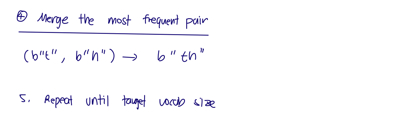
The BPE loop keeps merging the most frequent adjacent pair until the target vocabulary size is reached.
BPE encoding
Encoding is different from training.
Start from bytes
No corpus-level counting happens during encoding.
Apply earliest learned merges
Merge only pairs that exist in merge_ranks, in learned priority order.
During encoding, the merges are already learned. We do not count frequencies again. For each pre-token:
- Start from single-byte pieces.
- List adjacent pairs currently present.
- Keep only pairs that exist in the learned
merge_ranks. - Merge the earliest learned pair.
- Repeat until no learned pair applies.
- Map final byte pieces to token IDs.
pieces = [bytes([b]) for b in token_bytes]

while True:
    pairs = [(pieces[i], pieces[i + 1]) for i in range(len(pieces) - 1)]
    valid_pairs = [pair for pair in pairs if pair in merge_ranks]

    if not valid_pairs:
        break

    best_pair = min(valid_pairs, key=lambda pair: merge_ranks[pair])
    pieces = merge_everywhere(pieces, best_pair)
Special tokens add one more rule: split them out first. If the text contains <|endoftext|>, we encode that whole string as one ID, then run normal BPE only on the surrounding text.
text <-> token IDs. The embedding layer decides token ID -> learned vector. Same integer ID, two different jobs. II. Embeddings and PyTorch shape conventions
After tokenization, the model sees integer IDs:
token_ids = [[41, 93, 17, 10]]
The embedding layer is just a learned lookup table:
\[E \in \mathbb{R}^{V \times D}\]where $V$ is vocab size and $D$ is model width. If token ID 41 appears, the model takes row 41 of E.
class Embedding(torch.nn.Module):
    def __init__(self, vocab_size, d_model):
        super().__init__()
        self.weight = torch.nn.Parameter(torch.empty(vocab_size, d_model))

    def forward(self, token_ids):
        return self.weight[token_ids]
So the flow is:
\[[B,L] \to [B,L,D]\]The other important shape convention is linear layers. Papers often write $Wx$ using column vectors. PyTorch usually stores activations as row/batched vectors:
\[x \in \mathbb{R}^{\ldots \times d_{\text{in}}}\]So we store:
\[W \in \mathbb{R}^{d_{\text{out}} \times d_{\text{in}}}\]and compute:
y = x @ W.T
x @ W.T. III. The Transformer block
The block I implemented is a pre-norm decoder block:
Normalize before each sublayer, then add the residual path back in.
Pre-norm means we normalize before the attention/FFN sublayer, then add the residual connection.
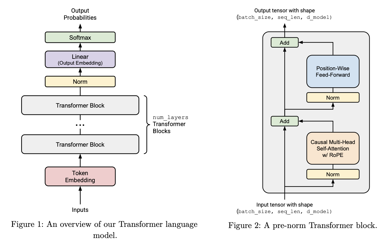
Transformer LM overview and pre-norm Transformer block.
RMSNorm
LayerNorm subtracts the mean and rescales. RMSNorm only rescales by the root mean square:
\[\text{RMS}(x) = \sqrt{\frac{1}{D}\sum_i x_i^2 + \epsilon}\] \[\text{RMSNorm}(x)_i = \frac{x_i}{\text{RMS}(x)} g_i\]The learnable scale $g$ has shape [d_model]. It broadcasts across [batch, sequence, d_model].
Multi-head attention shape flow
The packed projection gives Q/K/V in model width:
Then we split the final feature dimension into heads:
Q = q_proj(x).reshape(B, L, H, d_k)
K = k_proj(x).reshape(B, L, H, d_k)
V = v_proj(x).reshape(B, L, H, d_k)
Then transpose so attention runs over sequence length inside each head:
Q = Q.transpose(-3, -2)  # [B, H, L, d_k]
K = K.transpose(-3, -2)
V = V.transpose(-3, -2)
The attention matrix is [B, H, L, L], where each row says which previous tokens that position reads from.
After attention, we reverse the shape path:
out = attention(Q, K, V)          # [B, H, L, d_k]
out = out.transpose(-3, -2)       # [B, L, H, d_k]
out = out.reshape(B, L, D)        # [B, L, D]
SwiGLU
SwiGLU is the feed-forward block:
\[\text{SwiGLU}(x) = W_2(\text{SiLU}(W_1x) \odot W_3x)\]In PyTorch row-vector shape:
gate = silu(x @ W1.T)    # [..., d_ff]
value = x @ W3.T         # [..., d_ff]
hidden = gate * value    # [..., d_ff]
out = hidden @ W2.T      # [..., d_model]
The SiLU part is:
So the W1 branch is not just another plain projection. It makes a data-dependent gate for every token and every hidden feature. Large positive gate inputs mostly pass through, large negative gate inputs get pushed close to zero, and values near zero are softened smoothly. Then gate * value says: for this token, which expanded features from the W3 branch should be emphasized or muted before projecting back down?
IV. RoPE: position through rotation
Self-attention compares token vectors with dot products. Without positional information, the model knows which tokens exist, but not where they occur. Absolute position embeddings attach a learned vector to index 0, 1, 2, and so on, but that has two limitations:
- positions beyond the trained context length have no learned vector,
- relative distance has to be learned indirectly.
RoPE takes a different route. It rotates query and key vectors by their token position.
One thing that confused me at first: this is not merging or rotating adjacent tokens. RoPE rotates adjacent feature dimensions inside one token’s Q/K vector.
If a single head has $d_k = 8$, then one query vector at position $i$ looks like:
\[q_i = [q_{i,0}, q_{i,1}, q_{i,2}, q_{i,3}, q_{i,4}, q_{i,5}, q_{i,6}, q_{i,7}]\]RoPE groups adjacent feature dimensions inside that vector: $(0,1)$, $(2,3)$, $(4,5)$, and $(6,7)$. The token-to-token interaction happens later, when the rotated queries and keys are used in $QK^\top$. RoPE itself is a within-vector rotation.
Dimension-pairing view for one head
For $d_k = 8$, the pair index $k$ chooses which two coordinates get one 2D rotation.
| Pair index | Feature dimensions inside one token vector | Angle used |
|---|---|---|
0 | (q[i, 0], q[i, 1]) | $\theta_{i,0}$ |
1 | (q[i, 2], q[i, 3]) | $\theta_{i,1}$ |
2 | (q[i, 4], q[i, 5]) | $\theta_{i,2}$ |
3 | (q[i, 6], q[i, 7]) | $\theta_{i,3}$ |
This is why x[..., 0::2] and x[..., 1::2] show up in the implementation: they split all even and odd coordinates into the paired coordinates that RoPE rotates.
Important detail:
For a 2D pair, the rotation matrix is:
\[R(\theta) = \begin{bmatrix} \cos\theta & -\sin\theta \\ \sin\theta & \cos\theta \end{bmatrix}\]The key identity is:
\[R(\alpha)^\top R(\beta) = R(\beta - \alpha)\]So if token $m$ gets rotation $R(m\theta)$, and token $n$ gets rotation $R(n\theta)$, their attention dot product becomes:
\[(R(m\theta)x)^\top (R(n\theta)y) = x^\top R((n-m)\theta)y\]That is the core RoPE idea. The attention score now depends on the relative offset $n-m$, not just the two content vectors. If both positions shift by the same amount $k$, the relative spacing stays the same.
Derivation: why the relative-position term appears
The trig identities I want to remember are:
\[\sin(\alpha)\sin(\beta) = \frac{1}{2}\left[\cos(\alpha-\beta)-\cos(\alpha+\beta)\right]\] \[\cos(\alpha)\cos(\beta) = \frac{1}{2}\left[\cos(\alpha-\beta)+\cos(\alpha+\beta)\right]\] \[\sin(\alpha)\cos(\beta) = \frac{1}{2}\left[\sin(\alpha+\beta)+\sin(\alpha-\beta)\right]\] \[\cos(\alpha)\sin(\beta) = \frac{1}{2}\left[\sin(\alpha+\beta)-\sin(\alpha-\beta)\right]\]For the rotation matrix:
\[R(\theta) = \begin{bmatrix} \cos \theta & -\sin \theta \\ \sin \theta & \cos \theta \end{bmatrix}\]we have:
\[R(\alpha)^\top = \begin{bmatrix} \cos \alpha & \sin \alpha \\ -\sin \alpha & \cos \alpha \end{bmatrix}\]Now multiply:
\[R(\alpha)^\top R(\beta) = \begin{bmatrix} \cos\alpha\cos\beta+\sin\alpha\sin\beta & -\cos\alpha\sin\beta+\sin\alpha\cos\beta \\ -\sin\alpha\cos\beta+\cos\alpha\sin\beta & \sin\alpha\sin\beta+\cos\alpha\cos\beta \end{bmatrix}\]Using angle-difference identities:
\[\cos(\beta-\alpha)=\cos\beta\cos\alpha+\sin\beta\sin\alpha\] \[\sin(\beta-\alpha)=\sin\beta\cos\alpha-\cos\beta\sin\alpha\]we get:
\[R(\alpha)^\top R(\beta) = \begin{bmatrix} \cos(\beta-\alpha) & -\sin(\beta-\alpha) \\ \sin(\beta-\alpha) & \cos(\beta-\alpha) \end{bmatrix} = R(\beta-\alpha)\]The reason the sign cleans up is that cosine is even and sine is odd:
\[\cos(-\theta)=\cos(\theta), \qquad \sin(-\theta)=-\sin(\theta)\]Now apply this to the RoPE dot product:
\[\text{RoPE}(x,m)^\top \text{RoPE}(y,n) = x^\top R(m\theta)^\top R(n\theta)y = x^\top R((n-m)\theta)y\]If both positions shift by the same amount $k$:
\[\text{RoPE}(x,m+k)^\top \text{RoPE}(y,n+k) = x^\top R((m+k)\theta)^\top R((n+k)\theta)y = x^\top R((n-m)\theta)y\]The same relative spacing produces the same relative rotation.
Full matrix idea
For a head dimension $d_k$, RoPE conceptually builds a block-diagonal matrix:
\[R_i = \begin{bmatrix} R_i^1 & 0 & 0 & \cdots & 0 \\ 0 & R_i^2 & 0 & \cdots & 0 \\ 0 & 0 & R_i^3 & \cdots & 0 \\ \vdots & \vdots & \vdots & \ddots & \vdots \\ 0 & 0 & 0 & \cdots & R_i^{d_k/2} \end{bmatrix}\]Each block rotates one pair of dimensions. Building this full matrix would be wasteful.
For one pair $k$ at token position $i$, the actual operation is:
\[\begin{bmatrix} q'_{i,2k} \\ q'_{i,2k+1} \end{bmatrix} = \begin{bmatrix} \cos(\theta_{i,k}) & -\sin(\theta_{i,k}) \\ \sin(\theta_{i,k}) & \cos(\theta_{i,k}) \end{bmatrix} \begin{bmatrix} q_{i,2k} \\ q_{i,2k+1} \end{bmatrix}\]So the first row of the rotation matrix gives the new even coordinate:
\[q'_{i,2k} = q_{i,2k}\cos(\theta_{i,k}) - q_{i,2k+1}\sin(\theta_{i,k})\]and the second row gives the new odd coordinate:
\[q'_{i,2k+1} = q_{i,2k}\sin(\theta_{i,k}) + q_{i,2k+1}\cos(\theta_{i,k})\]cos and -sin are not just being "applied to the even index." They are the first row of the 2x2 rotation matrix, so the new even coordinate is a combination of the old even and old odd coordinates. Instead, precompute:
\[\cos(\theta_{i,k}),\quad \sin(\theta_{i,k})\]for every position $i$ and pair index $k$, then apply the 2D rotation directly to even and odd coordinates.
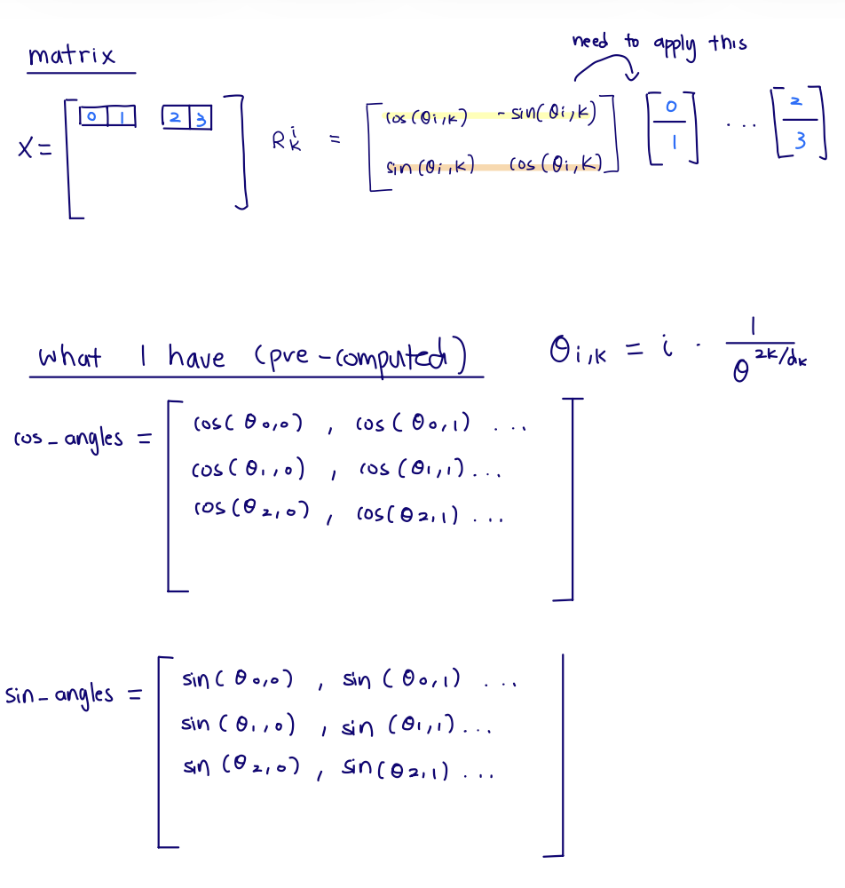
The precomputed RoPE tables store one row per token position and one column per even/odd feature pair.
new_odd = a * sin + b * cos
The full block matrix is conceptually helpful, but this pairwise formula is what the implementation actually wants.
old_even = x[..., 0::2]
old_odd = x[..., 1::2]

new_even = old_even * cos - old_odd * sin
new_odd = old_even * sin + old_odd * cos

out[..., 0::2] = new_even
out[..., 1::2] = new_odd
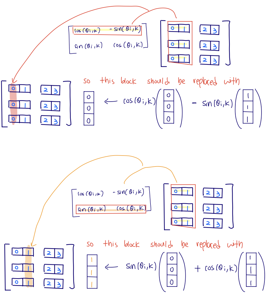
For each feature pair, the first row of the 2D rotation matrix produces the new even coordinate, and the second row produces the new odd coordinate.
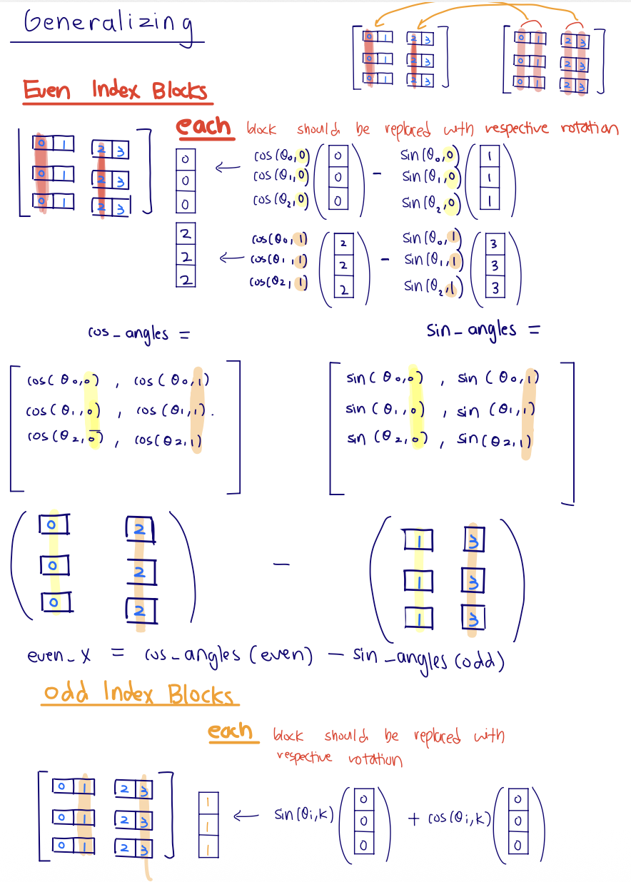
Generalizing the trick: split all even and odd feature columns, select the matching position rows from the precomputed sin/cos tables, then apply the same row-wise rotation everywhere.
The sin/cos values are not learned parameters. They are fixed buffers, reused across batches and layers:
self.register_buffer("cos_angles", cos_table, persistent=False)
self.register_buffer("sin_angles", sin_table, persistent=False)
A more complete version of the implementation looks like:
class RotaryPositionalEmbedding(torch.nn.Module):
    def __init__(self, theta: float, d_k: int, max_seq_len: int, device=None):
        super().__init__()

        positions = torch.arange(max_seq_len, device=device)      # [max_seq_len]
        pair_idx = torch.arange(d_k // 2, device=device)          # [d_k / 2]

        inv_freq = 1.0 / (theta ** (2 * pair_idx / d_k))
        angles = positions[:, None] * inv_freq[None, :]           # [max_seq_len, d_k / 2]

        self.register_buffer("cos_angles", torch.cos(angles), persistent=False)
        self.register_buffer("sin_angles", torch.sin(angles), persistent=False)

    def forward(self, x: torch.Tensor, token_positions: torch.Tensor) -> torch.Tensor:
        # x is usually Q or K with shape [B, H, L, d_k]
        # token_positions is usually [L], e.g. [0, 1, 2, ..., L-1]

        old_even = x[..., 0::2]  # [B, H, L, d_k / 2]
        old_odd = x[..., 1::2]   # [B, H, L, d_k / 2]

        cos = self.cos_angles[token_positions]  # [L, d_k / 2]
        sin = self.sin_angles[token_positions]  # [L, d_k / 2]

        out = torch.empty_like(x)
        out[..., 0::2] = old_even * cos - old_odd * sin
        out[..., 1::2] = old_even * sin + old_odd * cos
        return out
The reason this broadcasts is that cos and sin have shape [L, d_k / 2], which lines up with the last two dimensions of old_even and old_odd. The batch and head dimensions are leading dimensions, so PyTorch reuses the same position-angle table across batches and heads.
Then in attention:
Q = self.rope(Q, token_positions)
K = self.rope(K, token_positions)
# V is not rotated.
V. Training: many next-token predictions at once
The language modeling dataset is usually treated as one long stream of token IDs. Every step samples random windows:
Input window
Shifted targets
Causal attention makes each row a prefix task, so the whole chunk trains in parallel without future-token leakage.
x = tokens[start : start + L]
y = tokens[start + 1 : start + L + 1]
For a toy chunk:
x text:    the   cat   sat   on
y text:    cat   sat   on    mat
The Transformer keeps the sequence dimension:
\[[B,L] \to [B,L,D] \to [B,L,V]\]Each position gets its own next-token logits.
[the] -> cat, [the, cat] -> sat, [the, cat, sat] -> on, and so on. The causal mask prevents future-token leakage. The LM head is position-wise:
logits[:, i, :] = lm_head(hidden[:, i, :])
It is not cheating because the hidden state at position $i$ only contains information from tokens $\leq i$. The future blocking already happened inside causal attention.
Cross entropy
The model outputs logits, not probabilities:
\[\text{logits} \in \mathbb{R}^{B \times L \times V}\]For loss, flatten batch and sequence positions:
loss = cross_entropy(logits.reshape(-1, V), targets.reshape(-1))
That converts:
\[[B,L,V] \to [B \cdot L,V]\]and:
\[[B,L] \to [B \cdot L]\]The stable cross entropy identity I want to remember is:
\[\text{CE}(z,y) = \log\sum_j e^{z_j} - z_y\]and with the max trick:
\[\text{CE}(z,y) = m + \log\sum_j e^{z_j - m} - z_y, \quad m = \max_j z_j\]The reason subtracting $m$ is legal is that softmax does not change when every logit is shifted by the same constant:
\[\text{softmax}(z)_y = \frac{e^{z_y}}{\sum_j e^{z_j}} = \frac{e^{z_y-m}}{\sum_j e^{z_j-m}}\]because both numerator and denominator are multiplied by the same factor $e^{-m}$:
\[\frac{e^{z_y-m}}{\sum_j e^{z_j-m}} = \frac{e^{-m}e^{z_y}}{e^{-m}\sum_j e^{z_j}} = \frac{e^{z_y}}{\sum_j e^{z_j}}\]Then cross entropy is just negative log of the correct-token probability:
\[\begin{aligned} \text{CE}(z,y) &= -\log \frac{e^{z_y-m}}{\sum_j e^{z_j-m}} \\ &= -\left((z_y-m) - \log\sum_j e^{z_j-m}\right) \\ &= -z_y + m + \log\sum_j e^{z_j-m}. \end{aligned}\]So this is mathematically the same softmax probability. The exponentials are safer because the max shift guarantees:
\[z_j - m \leq 0 \quad\Longrightarrow\quad e^{z_j-m} \leq 1\]log. Perplexity is the same information on a more intuitive scale:
\[\exp(-\log p_{\text{correct}}) = \frac{1}{p_{\text{correct}}}\]Across many tokens, it is the inverse geometric mean probability assigned to the correct next token.
VI. Optimizer, schedule, clipping, checkpointing
The training-loop part I want to remember is how the scheduler and global gradient clipping show up in code:
for it in range(start_iter, args.max_iters):
    lr = get_lr_cosine_schedule(
        it=it,
        max_learning_rate=args.max_lr,
        min_learning_rate=args.min_lr,
        warmup_iters=args.warmup_iters,
        cosine_cycle_iters=args.cosine_cycle_iters,
    )

    for group in optimizer.param_groups:
        group["lr"] = lr

    x, y = get_batch(train_ids, args.batch_size, args.context_length, device)

    optimizer.zero_grad()
    logits = model(x)  # [B, L, V]
    loss = cross_entropy(logits.reshape(-1, vocab_size), y.reshape(-1))
    loss.backward()

    gradient_clipping(model.parameters(), args.max_grad_norm)
    optimizer.step()
For the cosine learning-rate schedule, the useful shape trick is:
\[s = \frac{t - T_w}{T_c - T_w}\]This maps the decay interval $[T_w, T_c]$ into progress $s \in [0,1]$. Then:
\[\frac{1}{2}(1 + \cos(\pi s))\]smoothly moves from 1 to 0, mapping $\alpha_{\max}$ to $\alpha_{\min}$.
Gradient clipping has to come after loss.backward() for a simple reason: backward() is the step that computes and stores the current gradients in each parameter’s .grad field. Before that, there is nothing from the current loss to clip.
The important detail is that this clipping is global. It calculates one L2 norm across the entire set of gradients:
\[\lVert g \rVert_2 = \sqrt{\sum_{\text{parameters }p}\sum_{\text{entries }r} g_{p,r}^2}\]Then it applies one shared scale factor to every gradient tensor if the norm is too large, meaning it goes beyond the chosen max_l2_norm.
def gradient_clipping(
    parameters: Iterable[torch.nn.Parameter],
    max_l2_norm: float,
) -> None:
    """Clip gradients in-place by global L2 norm."""
    eps = 1e-6

    grads = [p.grad for p in parameters if p.grad is not None]
    if len(grads) == 0:
        return

    total_sq_sum = sum(torch.sum(g**2) for g in grads)
    l2_norm = torch.sqrt(total_sq_sum)

    if l2_norm >= max_l2_norm:
        scale = max_l2_norm / (l2_norm + eps)
        for g in grads:
            g.mul_(scale)
AdamW then uses those clipped gradients inside optimizer.step(). AdamW still keeps per-parameter moment state like $m$, $v$, and $t$, but the clipping decision happened globally before the optimizer update.
AdamW also decouples weight decay from the gradient:
\[\theta \leftarrow \theta - \alpha \lambda \theta\]Resource accounting aha: why AdamW is 4P and where the FLOPs formulas come from
Let $P$ be the number of trainable scalar parameters. I sometimes wrote this as $N$, but I will use $P$ here so it does not collide with num_layers.
For the assignment architecture, ignoring biases:
\[P = 2VD + n_{\text{layers}}(4D^2 + 3DF + 2D) + D\]where:
- $V$ is vocab size,
- $D$ is
d_model, - $F$ is
d_ff, - $2VD$ is token embedding plus LM head,
- $4D^2$ is Q/K/V/output projection inside attention,
- $3DF$ is the three SwiGLU matrices,
- $2D$ is the two RMSNorm weights inside each block,
- the final $D$ is the last RMSNorm.
AdamW memory is easy to undercount because the optimizer is stateful. Around an optimizer step, the training run stores:
| Tensor kind | Size |
|---|---|
| parameters $\theta$ | $P$ floats |
| gradients $g$ | $P$ floats |
| Adam first moment $m$ | $P$ floats |
| Adam second moment $v$ | $P$ floats |
So parameter/gradient/AdamW persistent memory is:
\[P + P + P + P = 4P \text{ floats}\]With float32, that is:
\[4P \times 4 \text{ bytes} = 16P \text{ bytes}\]Equivalently, if $N$ means “number of parameters”, then this is $4N$ floats. The optimizer state alone is $2P$ floats, because it is just $m$ and $v$. Activations are extra and depend on batch size, context length, and which intermediate tensors are saved for backward.
For FLOPs, the one rule I want to keep in my head is:
\[[m,n] @ [n,p] \to [m,p] \quad\Rightarrow\quad 2mnp \text{ FLOPs}\]The factor of 2 is multiply plus add along the collapsed dimension $n$.
For one batch, let $B$ be batch size and $S$ be sequence length. Each Transformer layer has:
| Component | Shape reason | FLOPs |
|---|---|---|
| QKV projections | three $[BS,D] @ [D,D]$ multiplies | $6BSD^2$ |
| Attention scores $QK^\top$ | per head $[S,d_k] @ [d_k,S]$, summed over heads | $2BS^2D$ |
| Weighted values $AV$ | per head $[S,S] @ [S,d_k]$, summed over heads | $2BS^2D$ |
| Output projection | one $[BS,D] @ [D,D]$ multiply | $2BSD^2$ |
| SwiGLU FFN | $W_1$, $W_3$, and $W_2$ | $6BSDF$ |
Across all layers, multiply those layer costs by $n_{\text{layers}}$. The LM head adds:
\[2BSDV\]because it is $[BS,D] @ [D,V]$.
The quick intuition:
- FFN/projections scale like $S D^2$ or $SDF$,
- attention matrix multiplies scale like $S^2D$,
- so longer context makes attention grow much faster,
- bigger model width/depth makes projections and FFN heavier.
Finally, checkpointing is simply saving:
- model state,
- optimizer state,
- current iteration.
This matters because AdamW’s moment estimates are part of training state. Restarting with only the model weights is not the same as resuming training.
VII. Decoding: use the last row
Training predicts next-token logits at every position. Decoding only needs the final position.
Training
Every position contributes a next-token prediction.
Decoding
Sample one token, append it, then run the loop again.
Given prompt token IDs:
context_ids = generated_ids[-context_length:]
logits = model(context_ids)[..., -1, :]
For a prompt like Hi I am going, the model still returns one logits row per input position:
input tokens:   Hi        I        am        going
output rows:    next(Hi)  next(I)  next(am)  next(going)
decode uses:                                  ^ this row
During training, that last row would be compared against the actual next token from the dataset. During decoding, that next token is unknown, so we sample it from next(going), append it, and repeat.
Then decode one token:
if temperature <= 0:
    next_id = torch.argmax(logits)
else:
    probs = torch.softmax(logits / temperature, dim=-1)
    next_id = torch.multinomial(probs, num_samples=1)
Top-p sampling first sorts tokens by probability, keeps the smallest prefix whose probability mass exceeds $p$, renormalizes, and samples from that smaller set.
If the sampled token is <|endoftext|>, generation can stop. If it does not appear, generation stops at the chosen maximum token limit.
Final mental picture
The pieces feel much less mysterious when I separate the levels:
- Tokenizer: defines the discrete vocabulary and maps text to IDs.
- Embedding: gives each ID a learned vector.
- RoPE + attention: lets each position read previous positions with relative-position geometry.
- Transformer block: repeatedly mixes and transforms prefix information.
- LM head: maps every hidden row to vocab logits.
- Cross entropy: pushes up the correct next-token logit.
- Optimizer/training loop: turns those losses into stable parameter updates.
- Decoder: repeatedly reads the last-position logits and appends one sampled ID.
That is the building-block view I want to keep.
Enjoy Reading This Article?
Here are some more articles you might like to read next: