From Memory to Photonics: Solving the Next Bottleneck in AI Scaling

With Junho Park (Di Liang Lab, University of Michigan)

In the previous post, I used FlashAttention to show how the same attention calculation can run with less data transfer between high-bandwidth memory (HBM) and the smaller, faster memory on the processor.

When a model becomes too large for one GPU, or we want to train it faster, we distribute work across devices:

Tensor parallelism splits individual operations across devices, which exchange intermediate results.
Data parallelism runs model copies on different batches of data, then combines their gradients to update the model.
Pipeline parallelism places successive parts of the model on different devices and passes results between them.

These strategies give us more computing power, but they also create traffic between devices.

The next bottleneck is movement

Algorithms can reduce that traffic, but the remaining bits still need a physical link. Photonics uses light to carry and manipulate information. In an optical link, data travels on light through a fiber or a tiny channel on a chip called a waveguide.

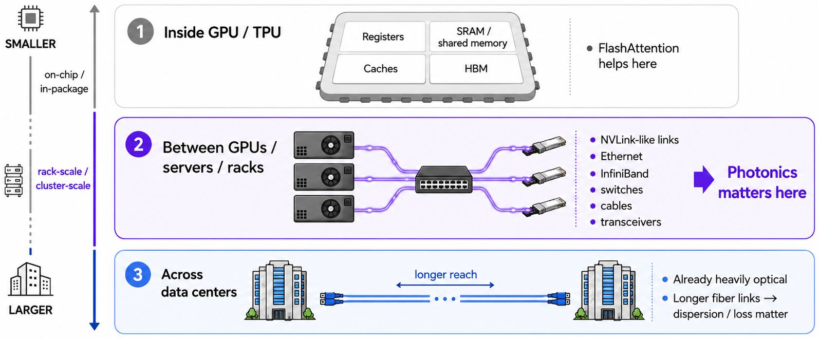
Hierarchy showing FlashAttention inside an accelerator and photonics between accelerators, servers, racks, and data centers

FlashAttention changes how data moves inside an accelerator. Photonics changes the physical link for data that must move between accelerators, servers, racks, and data centers.

One system, three bottlenecks

A processor can be limited by the speed of its calculations, its access to memory, or its connections to other processors:

Compute: How many useful operations can the accelerator perform per second?
Memory: How quickly can one accelerator obtain and reuse its local data?
Communication: How quickly can many accelerators exchange data and coordinate?

Which limit matters depends on the work and how it is divided. A useful starting point is how much math we do for each byte moved: enough work per byte can keep a processor busy while the next data arrives. The JAX Scaling Book’s roofline chapter develops this idea in more detail.

From chips to racks to data centers

Communication can take a larger share of runtime as work spreads across more processors and longer distances, especially when processors have to wait for each other’s results.

Three terms describe these connections, though their exact boundaries vary by vendor:

Scale up Connect more accelerators inside a tightly coupled system or rack.

Scale out Connect systems and racks into a larger cluster.

Scale across Connect data centers or campuses over longer distances.

Hand-drawn diagram showing scale-up, scale-out, and scale-across directions for data-center infrastructure

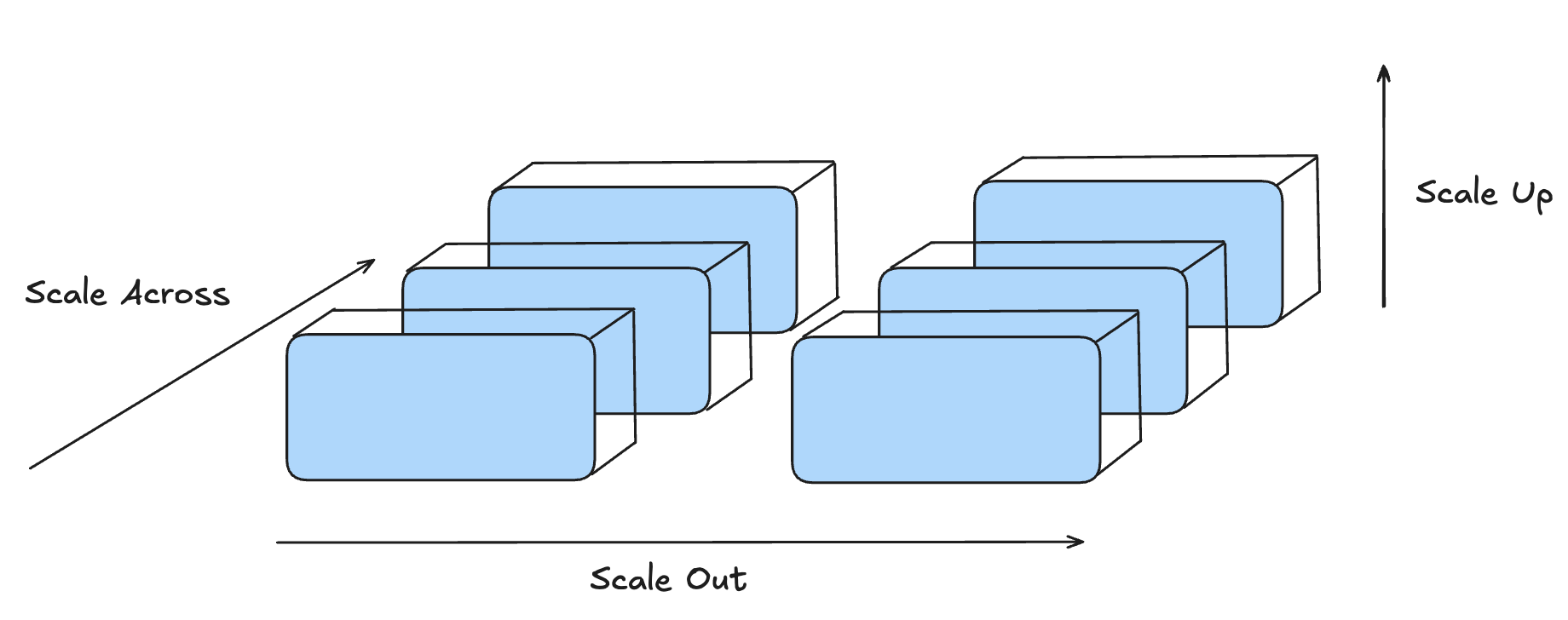
Connections within a system, between racks, and between data centers face different distance and bandwidth requirements.

Where copper gets expensive

Copper is widely used for short electrical links. It is inexpensive and works well over short distances.

The difficulty comes when we want more bits per second, longer connections, and less space for cables.

At higher signaling frequencies, more energy is lost in the conductor and surrounding insulating material. Signals weaken and become harder to distinguish. Extra circuits can compensate for distortion or restore the signal along the way, but they consume power and board space and produce heat.

As the data rate rises, passive copper cables, which have no powered signal-restoring electronics, become harder to use over long distances. Optical fiber can support much longer links.

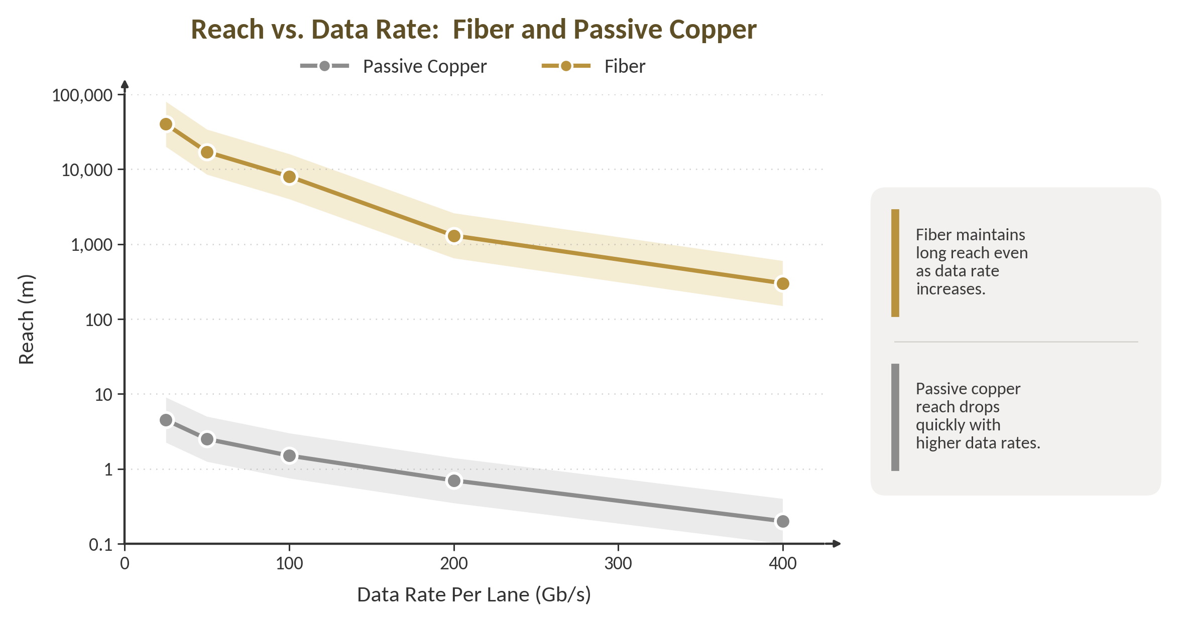
Illustrative comparison of reach versus data rate for passive copper and optical fiber; numerical values are not verified measurements

Illustrative trend only. The plotted values and shaded bands are not verified measurements or specification limits. Actual reach depends on the cable, transmitter, receiver, and signaling method.

The distance may be a few millimeters within a chip package, across a circuit board, or between racks. A package is the assembly that holds one or more chips and connects them to the rest of the computer.

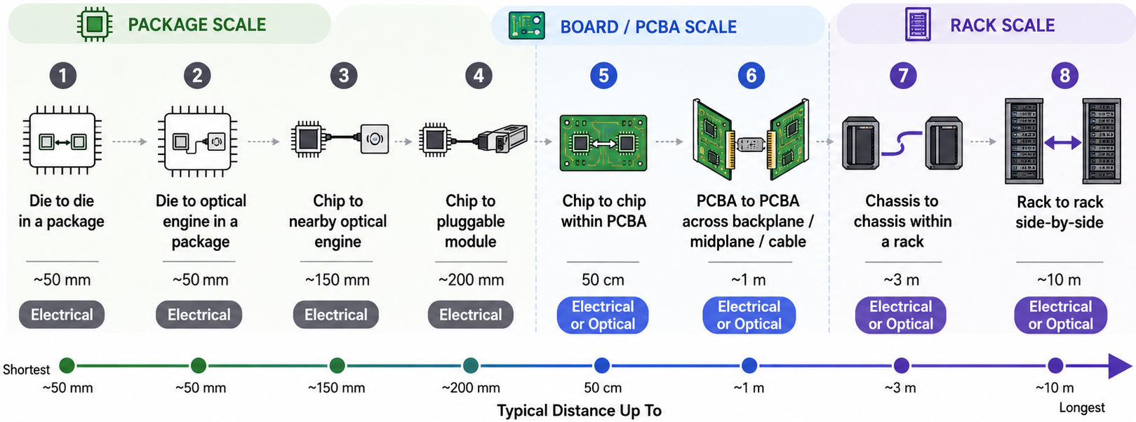
Hand-drawn diagram of interconnect lengths from package scale to board scale to rack scale

Interconnect distances from OIF's Next Generation CEI-224G Framework, Table 4 (source).

Electrical signals in copper also travel at a significant fraction of the speed of light. The advantage of optics is carrying large amounts of data over distance with manageable signal loss and energy use. There is no universal crossover point: the choice depends on the cable and the electronics at each end.

The optical boundary is moving toward compute

Data centers already use fiber for longer connections. The processors remain electronic, so data must be converted into an optical signal and back. Moving that conversion closer to the processor or network switch shortens the electrical part of the journey.

The direction is front-panel modules → optics on the circuit board → optics in the chip package. Bringing optics closer generally makes assembly, cooling, testing, and repair more demanding.

Optical I/O means optical input and output for a chip. It can use a small communication chip, or chiplet, in the processor’s package, so it overlaps with co-packaged optics (CPO). Intel’s optical I/O demonstration is one example.

Architecture	Where optics sits	Main benefit	Main cost
Pluggable optics	Replaceable module at the front panel	Mature and serviceable	Electrical signal must still reach the front panel
On-board optics	Optical conversion hardware near the processor or switch	Shorter electrical reach	Harder board assembly, cooling, and replacement
Co-packaged optics	Optical conversion hardware beside the processor or switch in one package	High bandwidth density and short electrical links	Shared heat, fiber attachment, testing, and repair
Optical I/O	Optical interface for a chip, often using a chiplet in the same package	Short electrical connection from compute to the optical interface	Integration with the processor, plus package and manufacturing constraints

An optical transceiver sends and receives data using light. Coherent’s image below shows the inside of a transceiver module and how similar components can be arranged around a switch or processor.

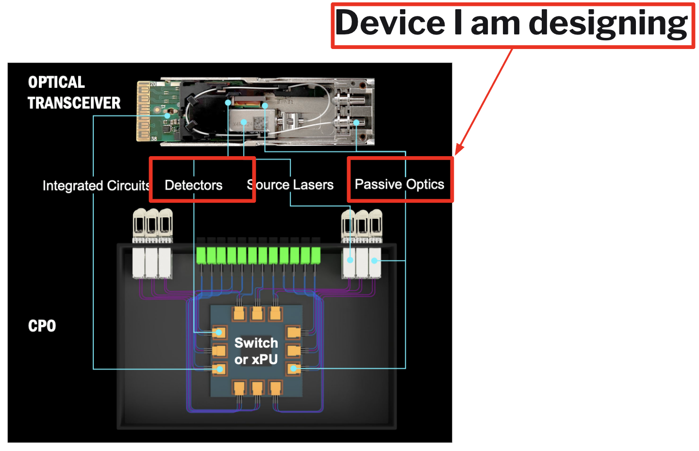
Annotated Coherent transceiver and CPO image with red boxes around detectors and passive optics, and an arrow pointing to passive optics as the device design focus

The passive-optics callout shows where devices such as our wavelength demultiplexers fit. Annotated from Coherent's Technology Innovation Briefing.

A front-panel module can usually be replaced on its own. When optics shares a package with an expensive processor, a faulty component may require more extensive repair. The design also has to account for the processor’s heat and the precise alignment needed to get light into and out of the fibers.

Two measurements help compare the options:

Energy per bit: How much total energy does the link spend to move one bit? Lower is better.
Shoreline bandwidth density: How much bandwidth can cross each millimeter of package edge? Higher is better.

Energy per bit must include the whole link: generating light, putting data onto it, detecting it, processing the signal, and controlling temperature. Light lost at connections can require more laser power.

For each distance and connection layout, the practical question is which link should become optical first, not when everything becomes optical.

How an optical link works

An optical link follows this path:

electrical data
    -> put data onto light (modulation)
    -> carry the light through a waveguide or fiber
    -> detect the light and recover the signal
    -> electrical data

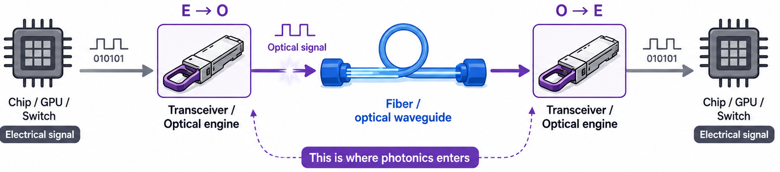
Diagram showing electrical-to-optical conversion, optical transmission through fiber, and optical-to-electrical conversion

The accelerator remains electronic. Photonics changes the communication path between endpoints.

A laser supplies the light, and a modulator changes it according to the electrical data. A detector at the receiving end converts the arriving light into an electrical signal.

One common design, a Mach-Zehnder modulator, splits light into two paths and recombines them. A voltage changes how light travels through one or both paths, shifting the relative timing of the waves, called their phase. When the waves meet again, they reinforce or cancel each other to different degrees. The resulting change in brightness carries the signal.

Silicon can guide light and is compatible with established chip manufacturing, but it is inefficient at emitting light. A practical system may bond a light-emitting material, such as indium phosphide, onto the silicon device, or supply light from a separate laser.

Wavelength is an extra axis

Light can carry separate data streams at different wavelengths. Think of them as different colors, although the wavelengths used here are typically infrared and invisible to us. Wavelength-division multiplexing (WDM) combines those streams onto one waveguide or fiber. A multiplexer, or mux, combines the wavelengths; a demultiplexer, or demux, separates them at the other end.

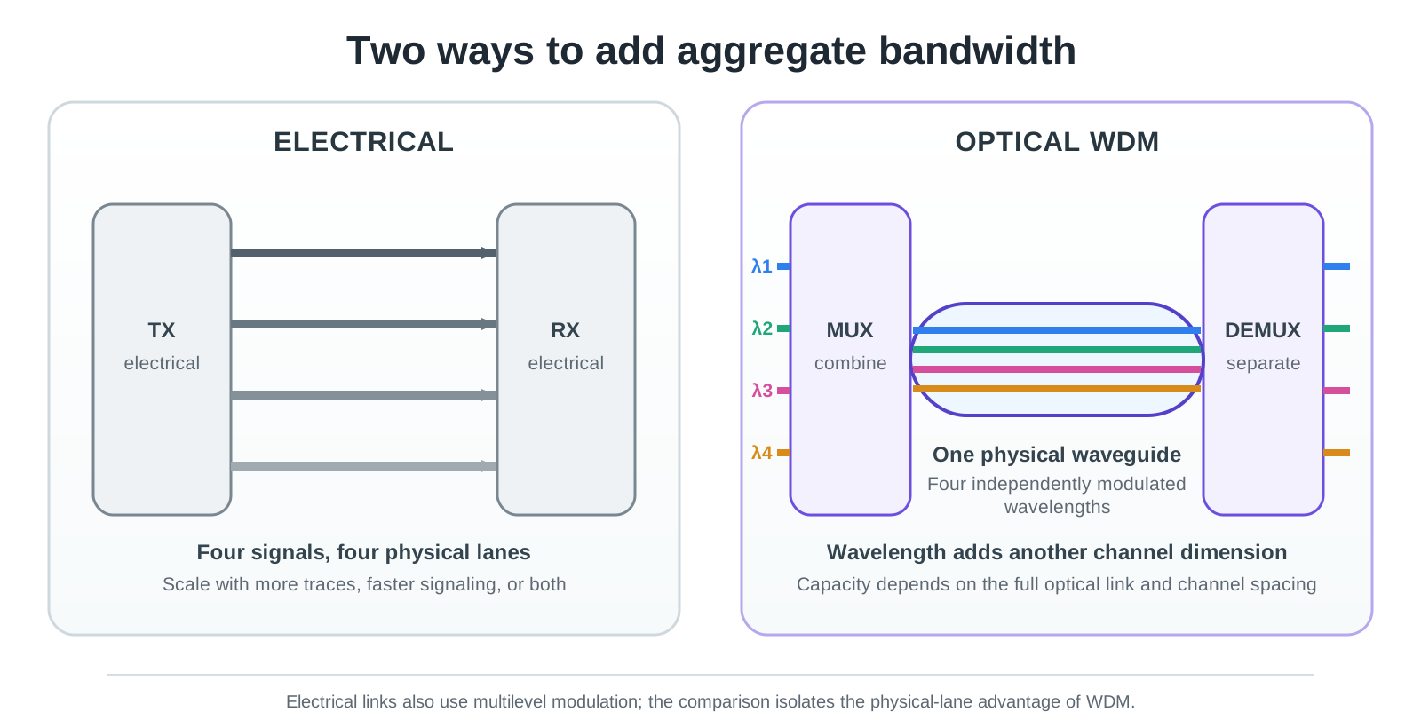
Electrical links often scale through faster signaling, more lanes, or both. WDM adds independently modulated wavelengths to one physical optical path.

Electrical links also carry more information through multiple voltage levels or frequency channels. WDM adds optical channels without needing a separate fiber or waveguide for each one.

Optical mux and demux components can also be passive: they can combine and separate wavelengths without active switching power. Their shapes and materials do the separating, but some light is lost along the way. This is called insertion loss, and compensating for it can require more laser power. Temperature changes can also shift which wavelengths a filter passes, so some designs need heating or tuning to stay aligned.

Those channels share a path, but the hardware that combines and separates them still needs space.

Photonics has a density problem too

In integrated photonics, the mux and demux are physical structures on a chip. Other components split light between paths, filter wavelengths, or guide it around bends. Together, they take up area.

Many photonic components are much larger than electronic transistors. Their dimensions depend on the wavelength of light, how tightly the material can confine it, and how far it needs to travel for the device to work. Shrinking a device means finding a shape that can still control the light in less space.

The package has limited space for these components and for the connections that carry signals out. Smaller muxes, demuxes, and splitters can leave room for more optical channels or other functions.

Fiber connections, electronics, optical losses, and heat can still limit bandwidth. But when device area is a constraint, a smaller design helps. Inverse design gives us a way to search for those smaller shapes.

What inverse design actually does

Conventional device design often starts with a familiar shape, such as a branching waveguide that splits light between two outputs. An engineer simulates it, changes a few dimensions, and repeats.

With inverse design, we specify the behavior we want and let an algorithm search for a shape. For example, we might ask it to send one wavelength to the upper output and another to the lower output, losing as little light as possible and keeping it out of the wrong port. A simulation predicts how light travels through each proposed shape.

The algorithm uses a gradient to decide which small changes should improve the result. The adjoint method can calculate these gradients across thousands of adjustable regions using a small number of simulations, rather than testing each region separately. It then adjusts the shape and repeats. The SPINS inverse-design framework paper explains the method in more detail.

This search can produce compact devices that would be hard to draw by intuition alone. The next step is making them.

From simulated designs to fabricated devices

An optimized shape may contain tiny holes, narrow bridges, or isolated islands of material. Some features are hard to manufacture consistently; others change the optical response significantly if their dimensions shift even slightly.

The steps that print and etch a pattern onto a chip cannot reproduce every boundary perfectly. Manufacturing constraints can be included during optimization, but a design that works in simulation still needs to be fabricated and tested.

Finding the design takes time, too. Simulations are expensive, and different starting shapes can lead to different results. Even after a search succeeds, it may be difficult to tell which features are essential and which could be simplified.

Previous designs and experiments can help us choose better starting shapes, identify sensitive features, and test changes that make a device easier to manufacture.

Where our work fits

Our work explores three connected ways to improve this design process:

Learn: reuse prior optimization efforts

We train a generative model on previous designs so a new search can start from what earlier optimization runs have learned.

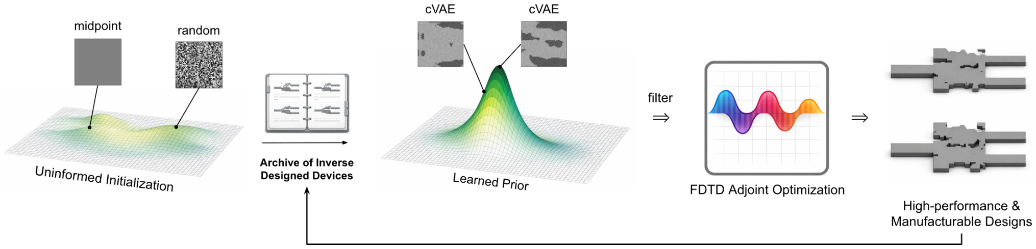
Pipeline comparing uninformed initialization with cVAE learned priors followed by FDTD adjoint optimization

A generative model proposes starting shapes from previous designs. Simulations then refine their optical performance.

Understand: identify feature sensitivity

We test which parts of a design matter most by making devices with deliberate, localized edits in predicted sensitive regions and in a less sensitive region for comparison. The microscope images below show those controlled changes.

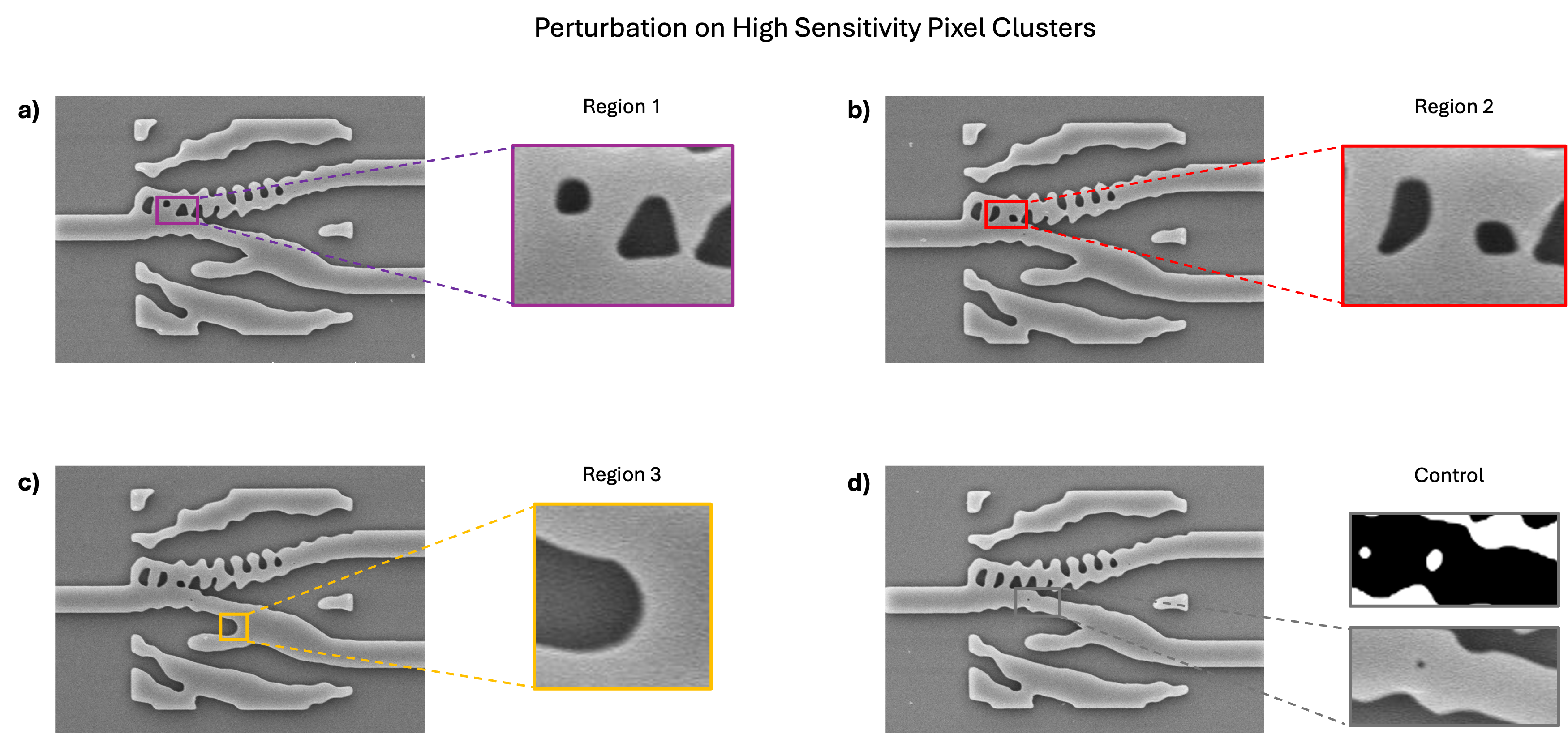
Electron microscope images of wavelength demultiplexers with deliberate local geometry changes in three predicted sensitive regions and a less sensitive control region

Sensitivity analysis identifies which deviations matter most for optical performance.

Refine: fabrication-friendly trimming

We use information from the optimization to rank edits that could simplify a layout. A new physics simulation checks that each accepted change preserves the required performance.

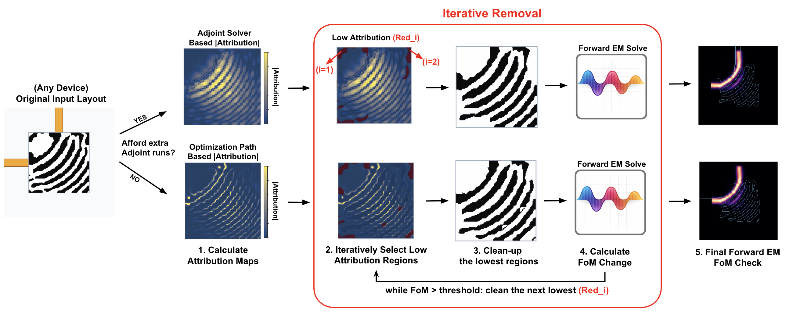
Workflow for solver-native attribution and iterative geometry removal verified by forward electromagnetic simulations

Candidate regions are removed one at a time, with simulations checking whether the device still meets its performance target.

These projects include one APL Engineering Physics paper and two papers accepted for IEEE Photonics Conference 2026 oral presentations. We want to connect these steps so that each design and experiment helps improve the next.

Movement is part of the architecture

FlashAttention reduces the memory traffic needed for a calculation. Optical links carry the data that still has to move between processors. Both help keep computing hardware supplied with data.

Bringing optics closer to compute makes that connection shorter, but puts more pressure on device size, power, and manufacturing. Compact photonic devices are one part of making those links practical. Their value comes from how well they work in the complete system.