Training a Language Model from Scratch (Part 2: FlashAttention and Device Memory)

In the previous blog post, I went over the basic building blocks of the language model: tokenization, embeddings, RoPE, attention, etc.

But if I zoom into the attention part, the previous post mostly treated it as a clean equation:

That is the right mathematical object, but it hides a systems question: what actually happens when the computer tries to run this equation?

This post is about that missing layer. Not just “what is attention?”, but why naive attention becomes memory-heavy, why softmax can be slower than the FLOP count makes it look, and why FlashAttention is such a nice algorithmic trick.

Profiling first

Some things we can observe from a profiling timeline:

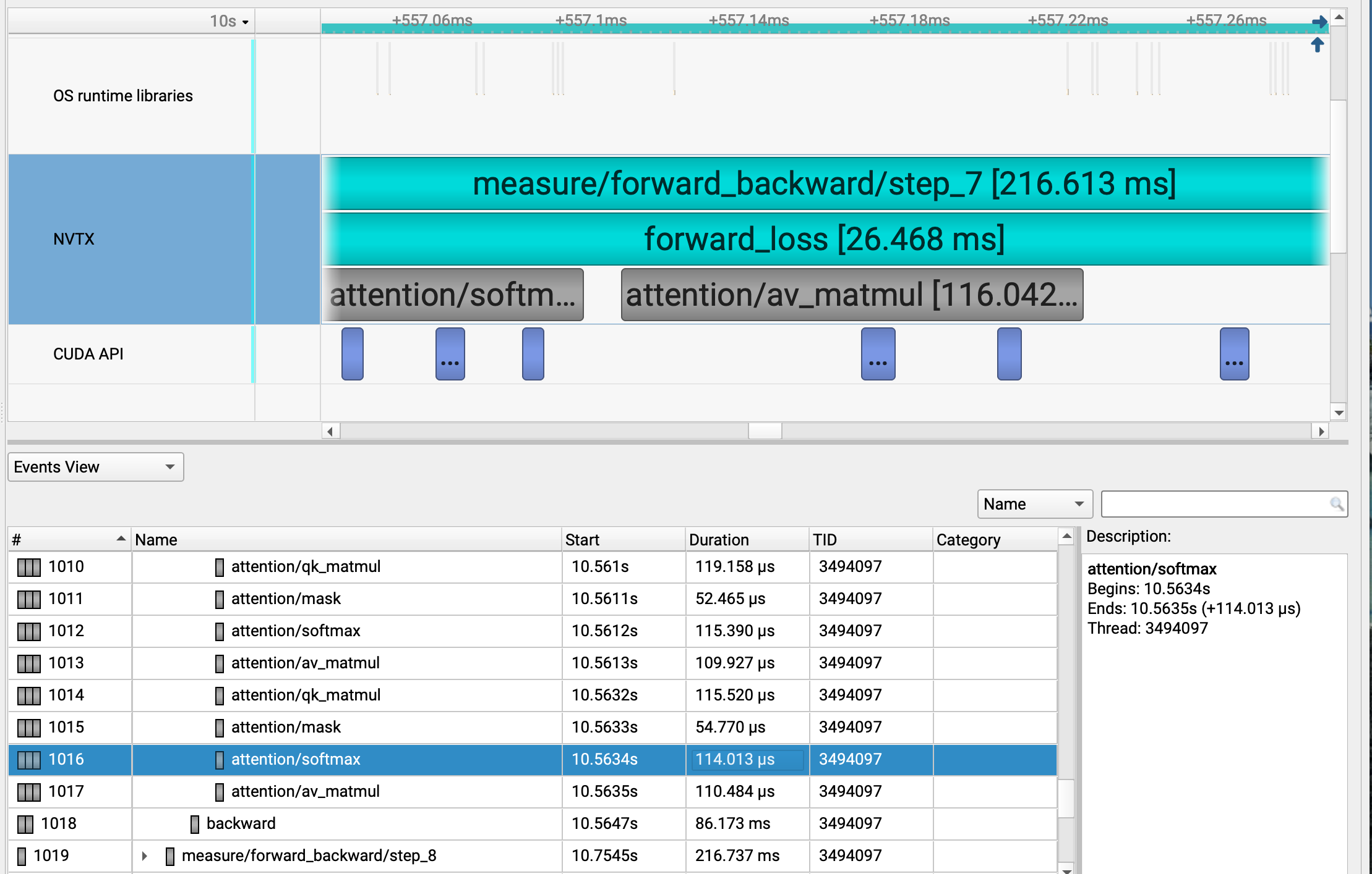
Profiling shows that attention is not only matmul. Softmax can take a meaningful part of the timeline even though its FLOP count is much smaller than the matmuls.

The first useful split is that “expensive” is not one word.

For FLOPs, the obvious large operations are matrix multiplications. In attention, those are:

and:

where:

But wall-clock time is not only FLOPs. Operations like softmax can take a surprisingly long time because they are reduction-heavy and memory-traffic-heavy. Stable softmax has to scan a row for the max, exponentiate, sum, divide, and write the result. Also, those operations are not the nice specialized GEMM work that accelerators are extremely good at.

So, like traditional algorithms, we have two axes:

1. Speed
2. Memory

And for attention, memory becomes especially painful because naive attention materializes matrices shaped like:

where $N$ is the sequence length. That $N^2$ is the part that quietly turns long context into a problem.

Before FlashAttention

Before going into FlashAttention, there are a few common techniques that show up everywhere.

Mixed precision

Operator fusion

x = x - x.max(dim=-1, keepdim=True).values
num = torch.exp(x)
den = num.sum(dim=-1, keepdim=True)
y = num / den

Recomputation / checkpointing

The missing idea: IO-awareness

The techniques above are useful, but by themselves they are not fully IO-aware.

By IO-aware, I mean: the algorithm explicitly cares about how many times data moves between different levels of memory.

At a high level, the relevant memory hierarchy is:

A kitchen analogy

The key point is that we want to access HBM as little as possible and do as much work as possible while the relevant tiles are already in on-chip memory.

Imagine a chef making beef soup.

The storage room is HBM. The kitchen table is on-chip SRAM/shared memory. The chef’s hands are registers.

If the chef had to walk to the storage room after every tiny step, it would be terrible. Chop one vegetable, walk back and store it. Bring it out again. Add salt, walk back again. Take it out again. The chef’s feet would be burning at this point.

The natural question is: why not bring everything into the kitchen at once?

Because the kitchen is small, and the door is narrow.

In more concrete terms, the accelerator cannot fit the entire attention matrix in fast on-chip memory. It has to move tiles through registers/shared memory while the full tensors live in HBM.

That is basically the attention problem. In naive attention, we bring big chunks of Q, K, and V, compute the full $QK^\top$ matrix, write that to HBM, read it back for softmax, write probabilities back, read them again, then multiply by V.

For the notation below, I sometimes write $QK^\top$ without the $1/\sqrt{d}$ scale. The scale is still part of real attention.

The math is clean:

But the memory movement is ugly:

compute S -> write S to HBM
read S -> compute P -> write P to HBM
read P and V -> compute O -> write O

FlashAttention asks: can we avoid this back and forth?

FlashAttention in a nutshell

FlashAttention combines tiling, online softmax, and recomputation.

It does not approximate attention. The output is still:

The difference is how the algorithm is scheduled.

Instead of materializing the full $S$ and $P$ matrices in HBM, FlashAttention:

1. Loads a tile of Q.
2. Streams over tiles of K and V.
3. Computes local score blocks.
4. Maintains running softmax statistics per query row.
5. Accumulates the output numerator.
6. Writes only the final output and a small log-sum-exp vector.

In FlashAttention-2, the forward pass uses an outer loop over Q row blocks and an inner loop over K/V column blocks. The original FlashAttention paper also used tiling, but FlashAttention-2 changed the loop order and work partitioning to improve parallelism and reduce unnecessary shared-memory traffic.

Original attention vs FlashAttention-2 tiling

The easiest way to understand this is to visualize the matrix multiplications.

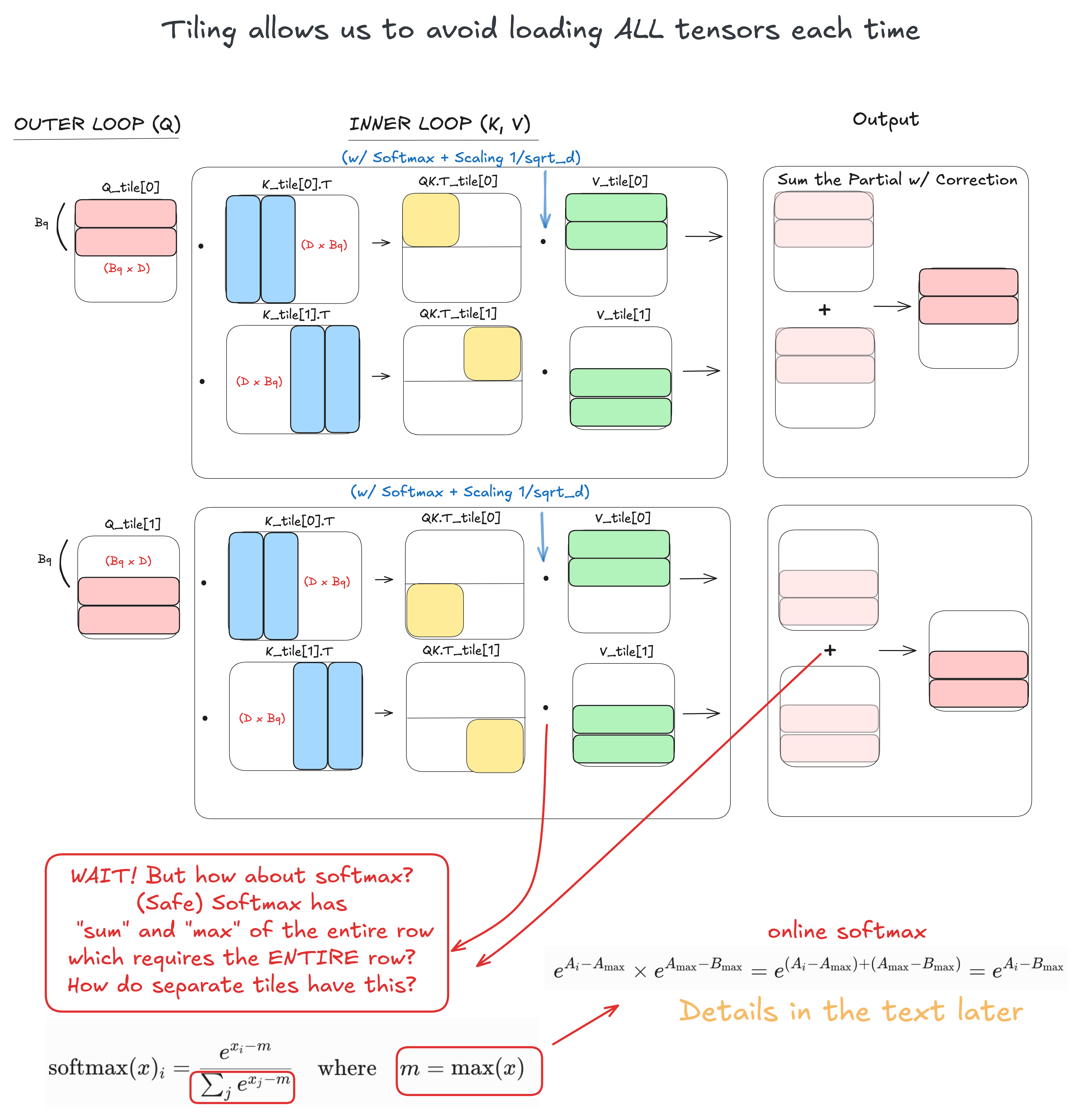
FlashAttention splits attention into row/column tile work instead of materializing the whole attention matrix. The output-side accumulation still needs online-softmax correction.

Conceptually, $QK^\top$ computes how much each query token attends to each key token. For a fixed query row, the softmax weights are spread across all key positions, and the output is a weighted sum of the matching V rows.

So we can split this row-wise work into chunks:

Q block i attends to K/V block 0
Q block i attends to K/V block 1
Q block i attends to K/V block 2
...

The problem is that softmax couples the entire row. We cannot just softmax each block independently and concatenate the answers. The denominator of softmax needs the whole row.

That is where online softmax enters.

Accumulating the partial output

For one query block, each K/V block gives a partial contribution to the final output.

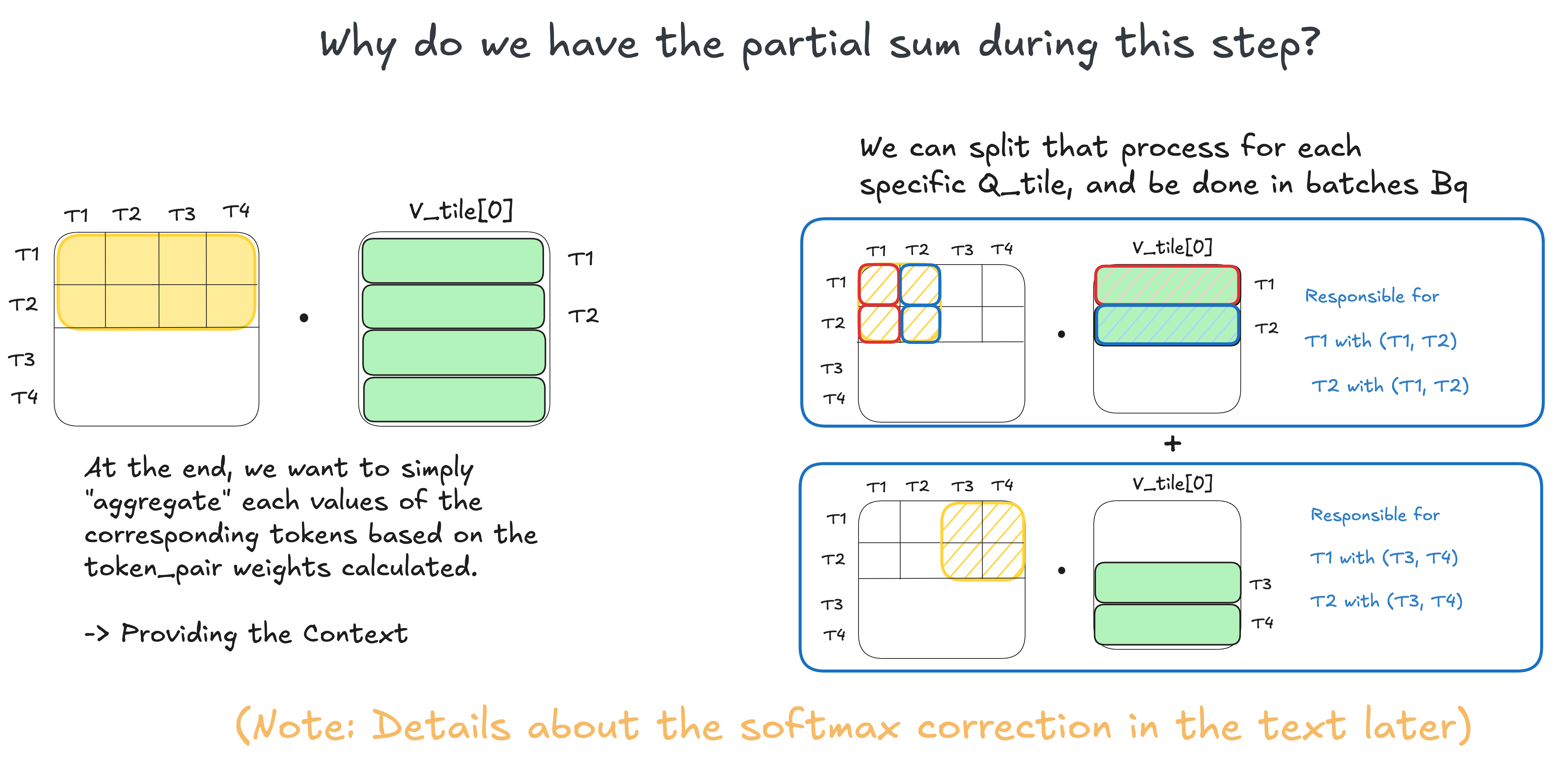
Each K/V tile contributes part of the final weighted sum. These partial contributions are rescaled with the running max and denominator before they are accumulated.

If the softmax denominator were not a problem, this would be easy:

Split over K/V blocks:

Safe / online softmax

Normally, stable softmax for one row is:

This requires knowing the max of the entire row.

But suppose the row is split into tile A and tile B.

Tile A has max $m_A$. Tile B has max $m_B$. The global max is:

If we processed tile A first using $m_A$, and later discover that $m_B$ is larger, the old tile A values were normalized with the wrong max. But this is fixable.

For an old value $x$ from tile A:

That tiny rescaling term is the whole trick:

So as we stream over blocks, we keep:

When a new block arrives:

Rescale the old denominator and numerator:

At the end:

That is the safe softmax trick in the streaming/tiled setting.

Connecting forward and backward with LSE

During backward, we do not want to have saved the full $S$ and $P$ matrices.

But we still need to recover $P$ blocks, because the gradient equations depend on softmax probabilities.

So what do we save?

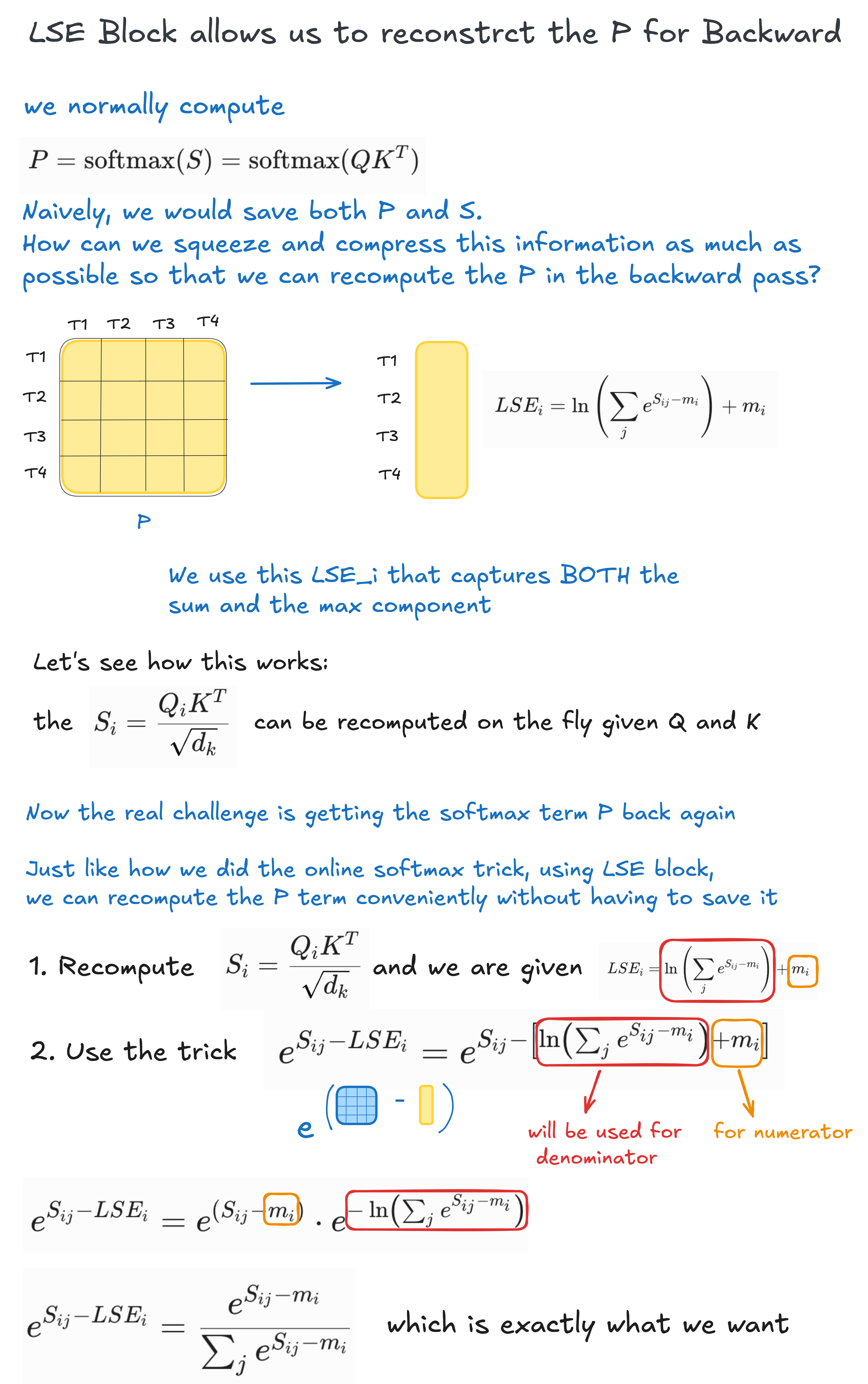
FlashAttention saves one log-sum-exp value per query row. The $+m_i$ term is the row-max stabilization term; the recovered probability is $e^{S_{ij} - L_i}$.

The compact value is log-sum-exp:

For numerical stability, this is computed as:

where $m_i$ is the row max.

Then during backward, if we recompute a score tile:

we can recover the softmax probability by:

This is the key step. We do not need the full old probability matrix. We only need Q, K, V, the output O, the upstream gradient dO, and the row-wise $L_i$ values. Then we recompute the probability block when that tile is already loaded.

One detail that matters: $L_i$ is not “left part denominator and right part numerator.” It is the log of the full softmax denominator, written in a stabilized way. Subtracting $L_i$ from a score gives exactly score minus log-denominator, and exponentiating gives the softmax probability.

Backward pass

Now we have the building blocks for the backward pass.

Naive attention might save large intermediate tensors like $S$ and $P$. FlashAttention avoids saving them. It saves or has access to:

Q, K, V
O
LSE
dO

Then it recomputes $S$ and $P$ block by block.

Backward streams over tiles again. It recomputes score/probability blocks, accumulates dK/dV for a K/V block, and updates dQ for matching query blocks.

The conceptual order is:

1. Recompute the local $P$ tile from $QK^\top$ and LSE.
2. Use $P$ to compute $dV$ and $dP$.
3. Use the softmax gradient to compute $dS$.
4. Use $dS$ to compute $dQ$ and $dK$.

In matrix form, the main equations are:

where $L$ is broadcast across the columns of each row.

Here $D$ is a row-wise correction term, often computed from $dO$ and $O$. The important point is that this softmax-gradient line is elementwise, not a matrix multiplication by $P$.

In the tiled backward pass, FlashAttention-2 conceptually flips the scheduling: it can hold a K/V block in the outer loop, stream through Q/dO/LSE/O blocks in the inner loop, accumulate dK and dV for that K/V block, and update dQ for each query block.

So:

outer loop: K/V block
inner loop: Q block

This feels natural because backward is going in reverse: we need to reconstruct the local $P$ block, use it to compute the local gradients, and aggregate the pieces.

Implementation notes: Triton

The next question is: how do we actually tell the computer to do this tiled movement?

PyTorch tensor code is great for expressing math, but it does not naturally give us control over “load this tile, keep this accumulator, avoid materializing this intermediate.” CUDA gives that control, but it is very low-level.

Triton sits in the middle. It gives a Python-like way to write GPU kernels where each program instance is basically a tile worker.

The Triton mental model:

In my naive forward kernel, the first grid axis chooses the Q tile, and the second grid axis chooses the batch:

pid_q = tl.program_id(axis=0)  # which Q tile
pid_b = tl.program_id(axis=1)  # which batch

q_rows = pid_q * BLOCK_M + tl.arange(0, BLOCK_M)
d_cols = tl.arange(0, BLOCK_D)

Then each program loads one Q tile:

q_ptrs = (
    q_ptr
    + pid_b * stride_qb
    + q_rows[:, None] * stride_qn
    + d_cols[None, :] * stride_qd
)

q_tile = tl.load(
    q_ptrs,
    mask=(q_rows[:, None] < Nq) & (d_cols[None, :] < D),
    other=0.0,
)

The kernel keeps the online softmax state in tile-shaped accumulators:

m = tl.full((BLOCK_M,), -float("inf"), tl.float32)
l = tl.full((BLOCK_M,), 0, tl.float32)
acc = tl.full((BLOCK_M, BLOCK_D), 0, tl.float32)

Then it streams over K/V blocks:

scores = tl.dot(q_tile, tl.trans(k_tile)) * scale

if IS_CAUSAL:
    scores = tl.where(q_rows[:, None] >= k_rows[None, :], scores, -float("inf"))

m_old = m
m_tile = tl.max(scores, axis=1)
m_new = tl.maximum(m_old, m_tile)

probs = tl.exp(scores - m_new[:, None])
correct_term = tl.exp(m_old - m_new)

l = correct_term * l + tl.sum(probs, axis=1)
acc = acc * correct_term[:, None] + tl.dot(probs, v_tile)
m = m_new

Finally:

out_tile = acc / l[:, None]
lse_tile = m + tl.log(l)

This is not production FlashAttention. It is a scrappy version I scribbled for learning.

The limitations are still important:

1. It is written for a simple shape like [B, N, D], not a fully optimized [B, H, N, D] production layout.
2. Real kernels tune block sizes carefully.
3. Real kernels have to care much more about dtypes, register pressure, shared memory, occupancy, causal masks, dropout, and backward.

There are definitely details I did not cover here. But writing this naive kernel made the main takeaway much clearer:

One last note on loop order

One detail that confused me at first was the loop order change from FlashAttention-1 to FlashAttention-2.

In FlashAttention-1, the forward pass roughly looked like:

for each K/V block:
    load K_j, V_j
    for each Q block:
        load Q_i and the running O_i, m_i, l_i state
        update the row-wise online softmax state
        write O_i, m_i, l_i back

So if we imagine the attention matrix, this schedule moves through column blocks first. That does not mean online softmax becomes impossible. FlashAttention-1 still computes the row-wise max, denominator, and output exactly. The issue is more about where the running row state lives and how often we touch it.

For a given Q row block, the values $m_i$, $\ell_i$, and the output accumulator need to be updated as more K/V blocks arrive. With K/V in the outer loop, those row states are revisited across column blocks. If we want more parallelism across the sequence dimension, that schedule is awkward because each row’s final softmax state depends on all the column-block contributions being combined correctly.

FlashAttention-2 flips the forward schedule:

for each Q block:
    keep m_i, l_i, and the output accumulator on-chip
    for each K/V block:
        update the row-wise online softmax state
    write O_i and LSE_i once

This lines up better with the row-wise nature of softmax. Each worker owns a block of query rows, streams across K/V blocks, and only writes the final output and LSE for that row block at the end. The row blocks are independent, so the forward pass gets cleaner parallelism over the sequence dimension.

The backward pass has a different reduction shape. There, using K/V blocks in the outer loop is natural because $dK$ and $dV$ collect contributions from many Q blocks. So the “column-wise” feeling is not wrong. It is just serving a different accumulation pattern.

Main takeaway

The core lesson is not only “FlashAttention is faster.”

The deeper lesson is that the same mathematical equation can have very different system behavior depending on what intermediate tensors are materialized.

Naive attention says:

make S
make P
make O

FlashAttention says:

stream tiles
keep online softmax stats
accumulate O
save LSE
recompute P blocks in backward

Same exact attention. Different memory story.

That is why IO-awareness matters.

References

• Stanford CS336: Language Modeling from Scratch, Spring 2025 — Assignment 2: Systems
• FlashAttention: Fast and Memory-Efficient Exact Attention with IO-Awareness
• FlashAttention-2: Faster Attention with Better Parallelism and Work Partitioning
• Triton fused softmax tutorial
• Triton program_id documentation
• Triton load documentation