From KV Cache to a State Matrix: Linear Attention and DeltaNet
In Transformer, Scaling, and Efficiency, I briefly covered methods such as grouped-query attention that reduce KV-cache memory. In the FlashAttention post, I looked at how IO-aware tiling avoids materializing the full attention matrix in HBM.
But now, let’s take a closer look at the cache itself.
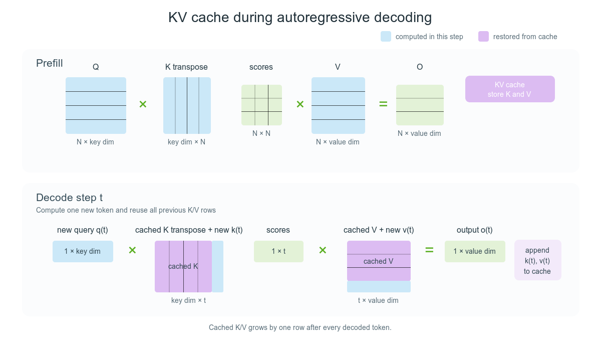
During prefill, the model computes K and V for all prompt tokens and stores them. Each decoding step reads the cached keys and values, computes one new q, k, and v, and appends the new k and v.
Figure recreated based on the KV-cache illustration in NVIDIA's Mastering LLM Techniques: Inference Optimization.
During autoregressive decoding, the keys and values of previous tokens do not change. We therefore cache them and reuse them for the next query. If the context contains $N$ tokens, the cache contains $N$ keys and $N$ values at every attention layer.
The KV cache is one of the main memory bottlenecks during decoding. It stores a key and value for every previous token at every layer, so even though its size grows linearly with $N$, it can become very large for long contexts. Each decoding step must also read this growing K/V history from HBM to compute attention for the new query, which makes decoding increasingly memory-bandwidth bound. This is separate from the $N^2$ attention-score matrix produced during prefill.
GQA reduces the number of key-value heads. PagedAttention manages how the cache is stored. Prefix caching reuses common prefixes. These are useful, but the cache still represents the context as an expanding list of key-value pairs.
Linear attention instead represents the context with a state matrix whose size does not depend on $N$.
From attention weights to a state matrix
Notation. We use column vectors: $q_t,k_t\in\mathbb{R}^{d_k\times1}$ and $v_t,o_t\in\mathbb{R}^{d_v\times1}$. Thus $v_t^\top$ is a row vector, and $k_tv_t^\top\in\mathbb{R}^{d_k\times d_v}$.
For this derivation, we start with the simplest unnormalized version of causal attention:
\[o_t = \sum_{j=1}^{t} (q_t^\top k_j)v_j.\]The left side of the figure shows this causal pattern. The new query $q_t$ can compare only with the keys from tokens $1$ through $t$, and those attention scores weight the corresponding values to produce $o_t$.
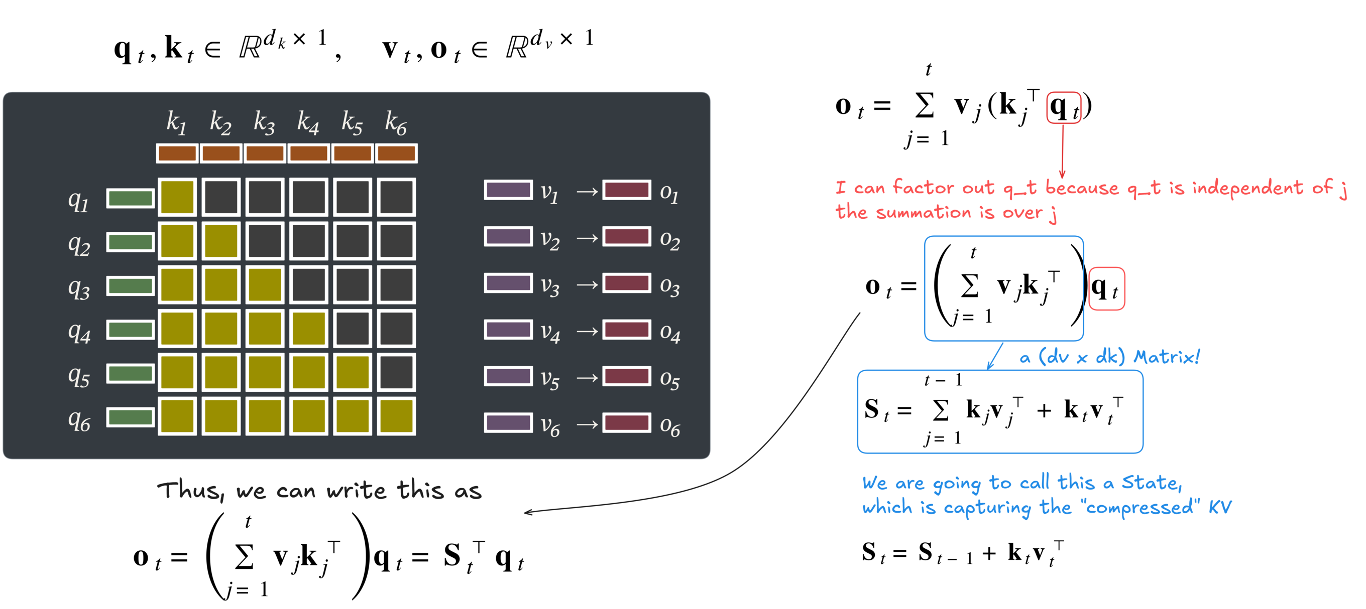
At step $t$, the query uses only the keys and values seen so far. The same products can be reordered into the fixed-size state $S_t$.
This and the later modeling diagrams are my own recreations based on the visual explanations in Jia-Bin Huang's lecture Beyond Softmax: The Future of Attention Mechanisms.
The upper-right side of the figure shows the same computation in a different order. Because $q_t$ does not depend on the summation index $j$, we can factor it out of the sum:
\[\begin{aligned} o_t &= \sum_{j=1}^{t}v_j(k_j^\top q_t) \\ &= \left(\sum_{j=1}^{t}v_jk_j^\top\right)q_t. \end{aligned}\]The matrix inside the parentheses has shape $d_v \times d_k$. We store its transpose as the state so that $S_t$ has shape $d_k \times d_v$:
\[S_t = \sum_{j=1}^{t}k_jv_j^\top \in \mathbb{R}^{d_k \times d_v}.\]Keeping $o_t$ as a column vector, the output is therefore:
\[o_t=S_t^\top q_t.\]The lower-right side of the figure separates the newest key-value pair from the previous prefix:
\[\begin{aligned} S_t &= \sum_{j=1}^{t-1}k_jv_j^\top+k_tv_t^\top \\ &=S_{t-1}+k_tv_t^\top. \end{aligned}\]Starting from $S_0=0$, each step updates the state with the current $k_t$ and $v_t$, then reads from it using $q_t$.
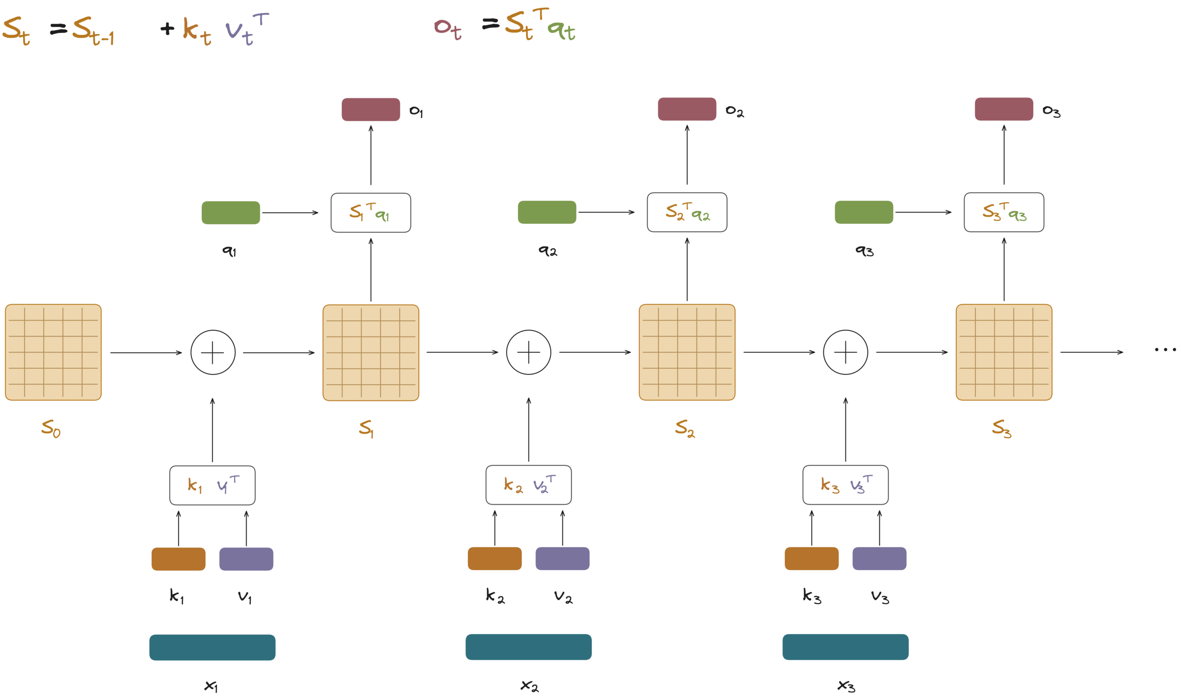
The basic linear-attention recurrence adds $k_tv_t^\top$ to the state, then reads $o_t=S_t^\top q_t$.
As shown in the diagram, $S_t$ is the state carried from one token to the next. At step $t$, we add the current association $k_tv_t^\top$, then apply the query $q_t$ to the updated state to obtain
\[o_t=S_t^\top q_t.\]The state remains $d_k \times d_v$ regardless of the context length. Instead of storing the key-value pairs separately, we compress them into this shared matrix.
This additive update has no explicit recency bias. A simple decay gate can reduce the previous state before adding the new association:
\[S_t = \gamma_tS_{t-1}+k_tv_t^\top, \qquad 0\leq\gamma_t\leq1.\]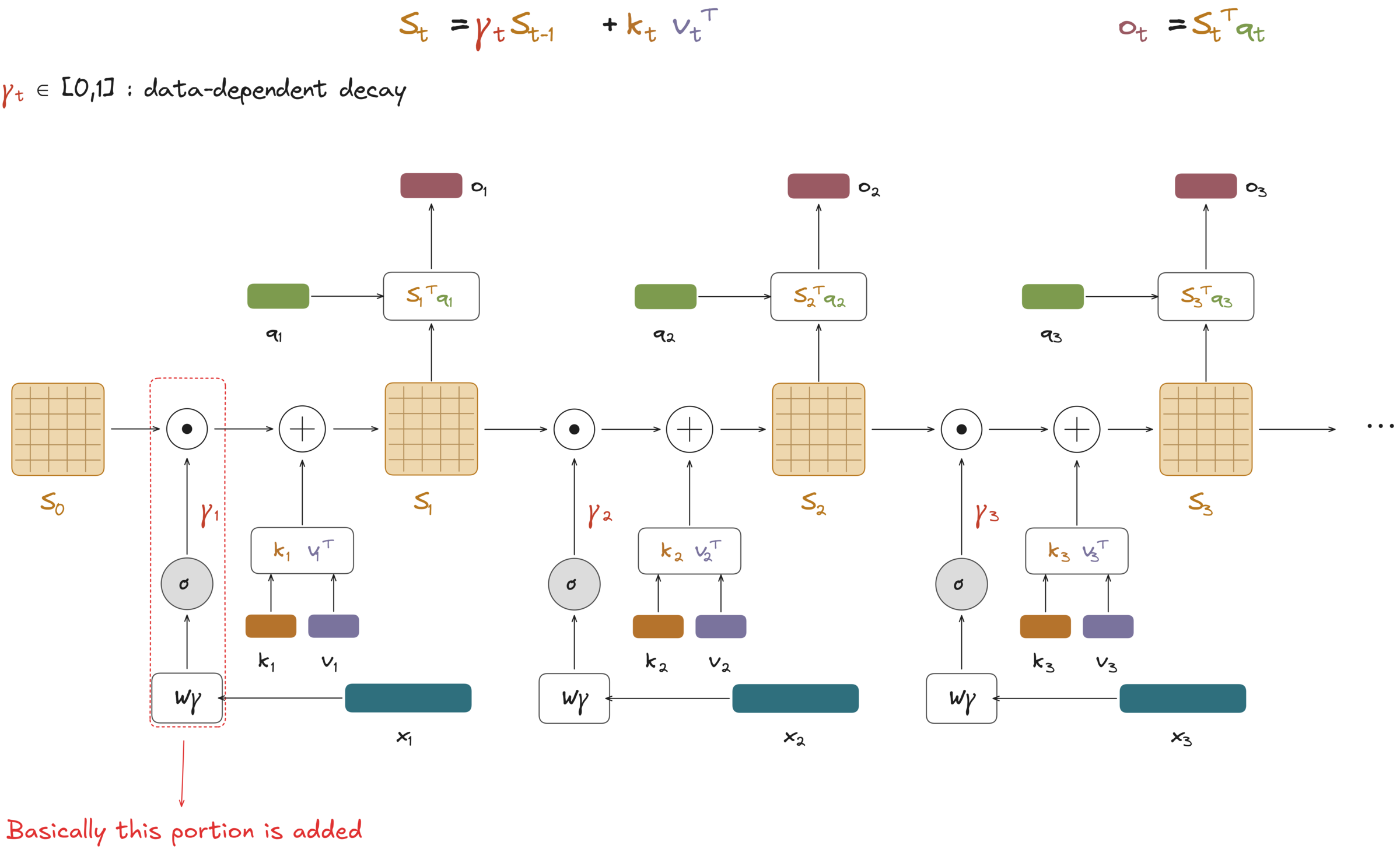
The data-dependent gate $\gamma_t$ scales the previous state before the new association is added.
Setting $\gamma_t=1$ recovers the original additive update.
Although this update is recurrent, training does not have to process the entire sequence one token at a time. Tokens can be grouped into chunks, with only the boundary state passed recurrently between them. We will return to this after introducing DeltaNet.
Associating keys and values
Now that we have the general picture of how the state is constructed and read, let’s take a closer look at how it associates each key with a value.
In softmax attention, the query is compared with the stored keys. The resulting attention weights determine how their associated values are combined.
Once we compress the key-value history into a state matrix, the question becomes:
How should we construct $S_t$ so that it works as a good associative memory?
Ideally, querying the state with a stored key $k_j$ should retrieve its associated value $v_j$:
\[S_t^\top k_j \approx v_j.\]More generally, if $q$ is similar to $k_j$, then $S_t^\top q$ should contain more of the corresponding $v_j$. This is exactly how the state read expands:
\[S_t^\top q = \sum_{j=1}^{t}v_j(k_j^\top q).\]This can also be viewed as a regression problem. The state $S$ is the parameter matrix of a linear function that maps a key to a predicted value:
\[f_S(k)=S^\top k.\]
The state matrix defines a linear map from a key $k$ to its predicted value $f_S(k)$.
To associate two vectors $a$ and $b$, we first use the negative dot-product loss:
\[\mathcal{L}^{\text{dot}}(a,b) = -\langle a,b\rangle.\]Substituting the value predicted from $k_t$ for $a$ and the target $v_t$ for $b$ gives:
\[\mathcal{L}^{\text{dot}}_t(S) = -\langle S^\top k_t,v_t\rangle.\]Here, $v_t$ is the value vector produced from the current token. It is the target of this small associative-memory update, not the ground-truth next token used to train the full language model.
Minimizing this loss encourages the value predicted from $k_t$ to have a large dot product with $v_t$. Its gradient is:
\[\nabla_S\mathcal{L}^{\text{dot}}_t(S) = -k_tv_t^\top.\]One gradient-descent step is:
\[\begin{aligned} S_t &= S_{t-1} -\beta_t\nabla_S \mathcal{L}^{\text{dot}}_t(S_{t-1}) \\ &= S_{t-1}+\beta_tk_tv_t^\top. \end{aligned}\]With $\beta_t=1$, this gives the same state recurrence derived above:
\[S_t=S_{t-1}+k_tv_t^\top.\]The state update is already a gradient update. Accumulating $k_tv_t^\top$ is equivalent to taking one online gradient step that teaches $S$ to associate $k_t$ with $v_t$.
This is an algebraic interpretation of the recurrence; inference does not run backpropagation or invoke an optimizer. It is why $S$ can be viewed as a fast-weight matrix: the model parameters remain fixed during inference, while the context updates $S$ at every token.
L2 loss and the delta rule
However, the negative dot-product loss used for this interpretation has an important limitation: it is not a distance between the value retrieved from the state and the target $v_t$. Since
\[\langle a,b\rangle = \lVert a\rVert\lVert b\rVert\cos\theta,\]the dot product can increase simply by increasing the vector norms. The update also ignores what the state already predicts for $k_t$; it adds the new association without correcting the old one.
To improve this, we can use the squared L2 distance between the value currently retrieved from the state and the target $v_t$. First, retrieve the old prediction:
\[\hat v_t^{\text{old}} = S_{t-1}^\top k_t.\]Then define the loss:
\[\mathcal{L}^{\text{L2}}_t(S) = \frac{1}{2} \lVert S^\top k_t-v_t\rVert_2^2.\]Its gradient at $S_{t-1}$ is:
\[\nabla_S\mathcal{L}^{\text{L2}}_t(S_{t-1}) = k_t(\hat v_t^{\text{old}}-v_t)^\top.\]Taking one gradient step gives:
\[\begin{aligned} S_t &=S_{t-1}-\beta_t\nabla_S \mathcal{L}^{\text{L2}}_t(S_{t-1}) \\ &=\boxed{ S_{t-1} +\beta_tk_t (v_t-\hat v_t^{\text{old}})^\top }. \end{aligned}\]This is the delta rule. Instead of always writing the full $v_t$, it writes the prediction error:
\[v_t-S_{t-1}^\top k_t.\]If the state already maps $k_t$ to $v_t$, the error is zero. If the stored association is wrong, the state is corrected in the direction of the error. The scalar $\beta_t$ controls the write strength.
Removing the old value and writing the new value
This L2-gradient form is less intuitive than the original outer-product sum. It helps to define:
\[v_t^{\text{new}} = (1-\beta_t)\hat v_t^{\text{old}} +\beta_tv_t.\]The delta update can then be written as:
\[\boxed{ S_t = S_{t-1} -k_t(\hat v_t^{\text{old}})^\top +k_t(v_t^{\text{new}})^\top. }\]Here, $\hat v_t^{\text{old}}$ is what the current state already retrieves for $k_t$. The new value $v_t^{\text{new}}$ blends that old prediction with the incoming $v_t$.
For the literal remove-and-replace interpretation, assume $\lVert k_t\rVert_2=1$. The algebraic delta update itself remains valid without this assumption.
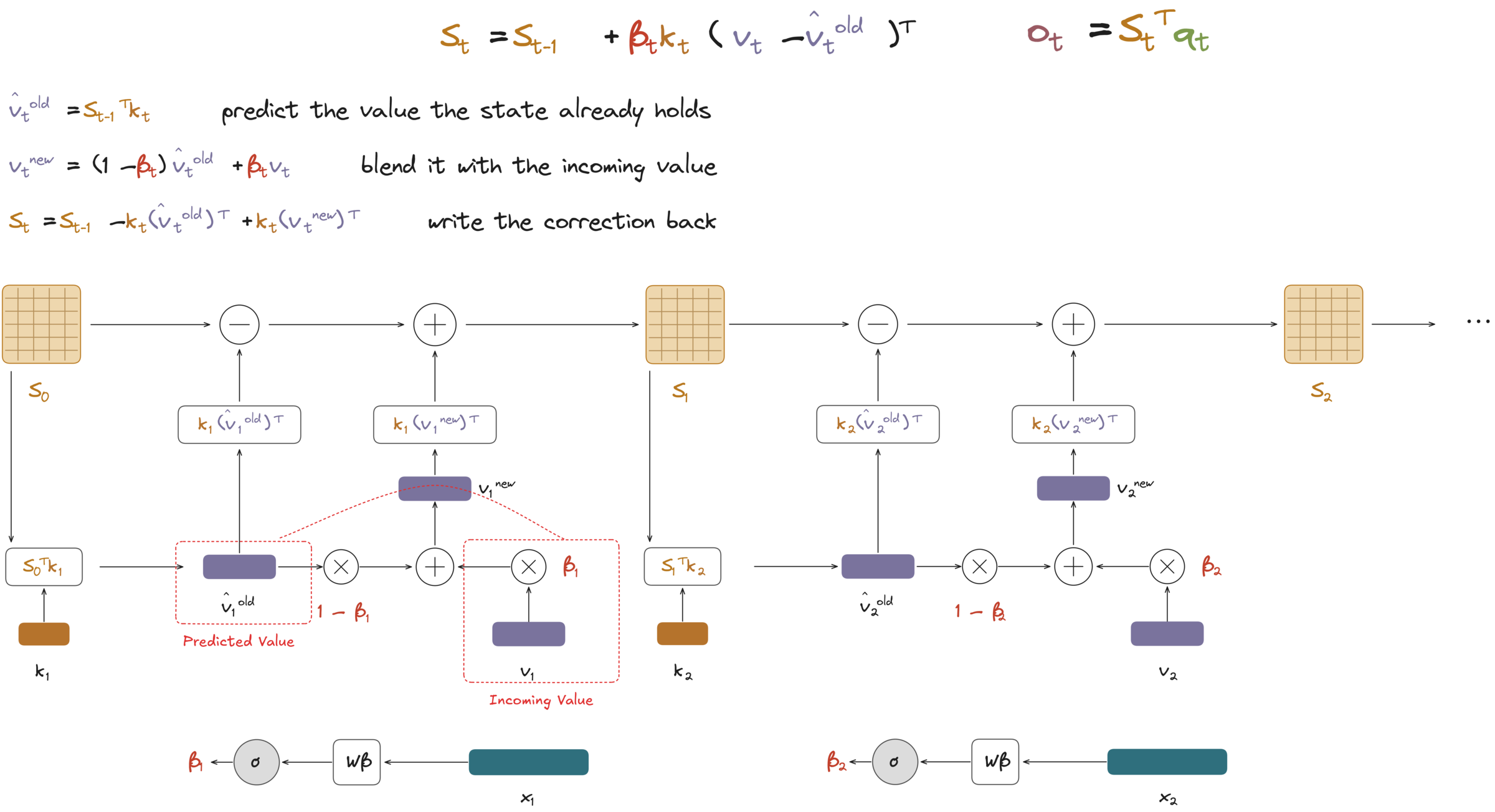
DeltaNet removes the value already associated with $k_t$ and writes the blended value $v_t^{\text{new}}$.
Because all associations share the same state matrix, correcting one key can also affect other keys that point in a similar direction.
Why the two forms are equivalent
Starting from the remove-and-write form:
\[\begin{aligned} S_t &= S_{t-1} -k_t(\hat v_t^{\text{old}})^\top +k_t(v_t^{\text{new}})^\top \\ &= S_{t-1} +k_t(v_t^{\text{new}}-\hat v_t^{\text{old}})^\top. \end{aligned}\]Now expand $v_t^{\text{new}}$:
\[\begin{aligned} v_t^{\text{new}}-\hat v_t^{\text{old}} &= (1-\beta_t)\hat v_t^{\text{old}} +\beta_tv_t -\hat v_t^{\text{old}} \\ &= \beta_tv_t +\hat v_t^{\text{old}} -\beta_t\hat v_t^{\text{old}} -\hat v_t^{\text{old}} \\ &= \beta_t(v_t-\hat v_t^{\text{old}}), \end{aligned}\]where the two copies of $\hat v_t^{\text{old}}$ cancel. Substituting this back gives the original delta-rule form:
\[S_t = S_{t-1} +\beta_tk_t (v_t-\hat v_t^{\text{old}})^\top.\]Chunkwise training for DeltaNet
Start from the delta update and substitute the value currently retrieved from the state, $\hat v_t^{\text{old}}=S_{t-1}^\top k_t$:
\[\begin{aligned} S_t &= S_{t-1} +\beta_tk_t(v_t-\hat v_t^{\text{old}})^\top \\ &= S_{t-1} +\beta_tk_t(v_t-S_{t-1}^\top k_t)^\top \\ &= S_{t-1} +\beta_tk_tv_t^\top -\beta_tk_tk_t^\top S_{t-1} \\ &= \underbrace{(I-\beta_tk_tk_t^\top)}_{A_t}S_{t-1} +\underbrace{\beta_tk_tv_t^\top}_{B_t}. \end{aligned}\]This has the state-space form:
\[S_t=A_tS_{t-1}+B_t.\]This is already a matrix equation, but it is still sequential across tokens: we cannot compute $S_1$ until we have $S_0$, then $S_2$ until we have $S_1$, and so on. The chunkwise goal is to compose several of these token-level affine updates into one equivalent update between chunk boundaries.
This kind of state unrolling may look familiar from EECS 16A.
Why use chunks?
Take a toy sequence with two tokens per chunk:
\[\text{chunk 1:}\qquad \boxed{S_0} \xrightarrow{A_1,B_1} S_1 \xrightarrow{A_2,B_2} \boxed{S_2}\] \[\text{chunk 2:}\qquad \boxed{S_2} \xrightarrow{A_3,B_3} S_3 \xrightarrow{A_4,B_4} \boxed{S_4}.\]Each arrow is one token update. The boxed states are the chunk boundaries passed from one chunk to the next. Within the first chunk,
\[\begin{aligned} S_1&=A_1S_0+B_1, \\ S_2&=A_2S_1+B_2 \\ &=\underbrace{A_2A_1S_0}_{\text{previous memory after two transitions}} +\underbrace{A_2B_1+B_2}_{\text{writes made inside the chunk}}. \end{aligned}\]The goal is therefore to compute the two underbraced parts directly at the chunk level: one describes how the chunk transforms the incoming memory, and the other collects the writes made inside it. The optional derivation below shows how both can be regrouped into block matrix operations.
The same pattern over more steps
\[\begin{aligned} S_3 &=A_3A_2A_1S_0+A_3A_2B_1+A_3B_2+B_3, \\ S_T &=(A_TA_{T-1}\cdots A_1)S_0 \\ &\quad+(A_TA_{T-1}\cdots A_2)B_1 \\ &\quad+(A_TA_{T-1}\cdots A_3)B_2 +\cdots+A_TB_{T-1}+B_T. \end{aligned}\]Each write $B_i$ is transformed by every later $A_j$ before it reaches $S_T$.
Optional note for me to review again: deriving the transition and write matrices
Compressing the previous-memory transition
The next goal is to express both grouped parts, $A_2A_1$ and $A_2B_1+B_2$, as matrix products. The useful structure is that every transition
\[A_t=I-\beta_tk_tk_t^\top\]differs from the identity only by the outer product $\beta_tk_tk_t^\top$. This outer-product matrix is called rank one because every one of its columns is a scaled copy of $k_t$; it acts only along the direction of $k_t$. The transition $A_t$ itself is not necessarily rank one.
The next step does not change the multiplication order. It only uses associativity to multiply the two middle vectors first:
\[(ab^\top)(cd^\top)=a(b^\top c)d^\top,\]Since $b^\top c$ is a scalar, multiplying two outer-product matrices produces another outer-product matrix instead of an unrelated dense term. To see how this helps, expand the first two transitions:
\[\begin{aligned} A_2A_1 &= (I-\beta_2k_2k_2^\top) (I-\beta_1k_1k_1^\top) \\ &= I -\beta_1k_1k_1^\top -\beta_2k_2k_2^\top +\beta_1\beta_2k_2(k_2^\top k_1)k_1^\top. \end{aligned}\]Because $k_2^\top k_1$ is a scalar, the cross term remains an outer product with $k_2$ on the left. This lets us group it with the other $k_2$ term and absorb both into a single factor $-k_2w_2^\top$. Preserving this outer-product form is what later lets us stack the factors into $K^\top W$. First, the term involving $k_1$ is
\[-\beta_1k_1k_1^\top = -k_1(\beta_1k_1)^\top,\]while the two terms involving $k_2$ become
\[\begin{aligned} &-\beta_2k_2k_2^\top +\beta_1\beta_2k_2(k_2^\top k_1)k_1^\top \\ &\qquad= -k_2 \left( \beta_2k_2 -\beta_1\beta_2(k_2^\top k_1)k_1 \right)^\top. \end{aligned}\]The vectors inside these two right-hand factors are what we name $w_1$ and $w_2$:
\[\begin{aligned} w_1&=\beta_1k_1, \\ w_2&=\beta_2k_2-\beta_1\beta_2(k_2^\top k_1)k_1. \end{aligned}\]These are not new model states; they simply collect the interactions created by multiplying the $A$ matrices. We can now write
\[A_2A_1 =I-k_1w_1^\top-k_2w_2^\top.\]Instead of keeping the two outer products separately, stack the vectors by rows:
\[K= \begin{bmatrix} k_1^\top \\ k_2^\top \end{bmatrix}, \qquad W= \begin{bmatrix} w_1^\top \\ w_2^\top \end{bmatrix}.\]Then the block matrix multiplication expands back into the two outer products:
\[\begin{aligned} K^\top W &= \begin{bmatrix} k_1 & k_2 \end{bmatrix} \begin{bmatrix} w_1^\top \\ w_2^\top \end{bmatrix} \\ &=k_1w_1^\top+k_2w_2^\top. \end{aligned}\]Therefore,
\[\boxed{A_2A_1=I-K^\top W.}\]The product $I-K^\top W$ summarizes how the two-token chunk transforms the memory that was already present in $S_0$.
Compressing the writes inside the chunk
Now consider the write part of the toy chunk (or the right part of the equation, lol):
\[S_2 = A_2A_1S_0 +\color{#d9534f}{\boxed{A_2B_1+B_2}}.\]The write contribution is not just $B_1+B_2$: the first write $B_1$ passes through the later transition $A_2$. Substitute
\[\begin{aligned} A_2&=I-\beta_2k_2k_2^\top, \\ B_1&=\beta_1k_1v_1^\top, \\ B_2&=\beta_2k_2v_2^\top. \end{aligned}\]Then expand:
\[\begin{aligned} A_2B_1+B_2 &= (I-\beta_2k_2k_2^\top) (\beta_1k_1v_1^\top) +\beta_2k_2v_2^\top \\ &= \beta_1k_1v_1^\top -\beta_1\beta_2k_2k_2^\top k_1v_1^\top +\beta_2k_2v_2^\top \\ &= \beta_1k_1v_1^\top -\beta_1\beta_2k_2(k_2^\top k_1)v_1^\top +\beta_2k_2v_2^\top. \end{aligned}\]The first term is $k_1u_1^\top$ if we define $u_1=\beta_1v_1$. Group the remaining two terms, which both have $k_2$ on the left, by defining
\[u_2=\beta_2v_2-\beta_1\beta_2(k_2^\top k_1)v_1.\]Stack these adjusted write vectors in the same order:
\[U= \begin{bmatrix} u_1^\top \\ u_2^\top \end{bmatrix}.\]The complete write part is then
\[\begin{aligned} A_2B_1+B_2 &=k_1u_1^\top+k_2u_2^\top \\ &=K^\top U, \end{aligned}\]The product $K^\top U$ summarizes the new writes made inside the chunk after accounting for how the second token modifies the first one. Compact WY repeats this regrouping across all $C$ tokens without materializing every intermediate state or matrix product.
Putting the chunk together
The optional derivation above compresses the two parts of the toy chunk into
\[A_2A_1=I-K^\top W, \qquad A_2B_1+B_2=K^\top U.\]For our two-token toy chunk, the direct block update is therefore
\[\boxed{ S_2=(I-K^\top W)S_0+K^\top U. }\]Now apply the same regrouping to a chunk of $C$ tokens. Let $S_{[c]}$ be the state before chunk $c$ and $S_{[c+1]}$ the state after it. Compact WY constructs chunk matrices $W_{[c]}$ and $U_{[c]}$ so that the entire chunk update becomes
\[\boxed{ S_{[c+1]} = \left(I-K_{[c]}^\top W_{[c]}\right)S_{[c]} +K_{[c]}^\top U_{[c]}. }\]Here, $K_{[c]}$ stacks the keys in the chunk. The first term carries the previous memory through all the delta transitions in that chunk. The second term combines all the new writes. It uses the transformed $U_{[c]}$ rather than the raw values $V_{[c]}$ because later tokens in the chunk modify earlier writes.
Only the boundary state passes recurrently from one chunk to the next; the work within each chunk is grouped into matrix operations that can run in parallel on the GPU.
Why DeltaNet may forget too slowly
Chunking changes how efficiently we compute the update, but it does not change what the update remembers.
The delta rule corrects the memory associated with the current key $k_t$, but it has no independent mechanism for weakening the rest of the state. As a result, associations written much earlier can remain even after they are no longer useful, and forgetting them may require many later updates involving related keys.
To address this, Gated DeltaNet adds a separate scalar forget gate $\alpha_t$. First decay the previous state:
\[\widetilde S_{t-1}=\alpha_tS_{t-1}.\]Then apply the delta update to the decayed state:
\[S_t = \widetilde S_{t-1} +\beta_tk_t (v_t-\widetilde S_{t-1}^\top k_t)^\top.\]The roles are separate: $\alpha_t$ can forget the state broadly, while $\beta_t$ controls the targeted key-value correction.
Connection to test-time training
Returning to the gradient interpretation, DeltaNet can be viewed as treating $S$ as the parameter matrix of a linear regression:
\[f_S(k)=S^\top k.\]The state is updated from the current context even during inference. In this sense, it behaves like a small model being trained online while the normal model parameters remain fixed.
This raises a more general question: does the state have to be a single linear map? Test-time-training methods extend this view by using a more expressive inner model and updating its parameters from the context. We will leave that extension for a later note.
Wrap-up
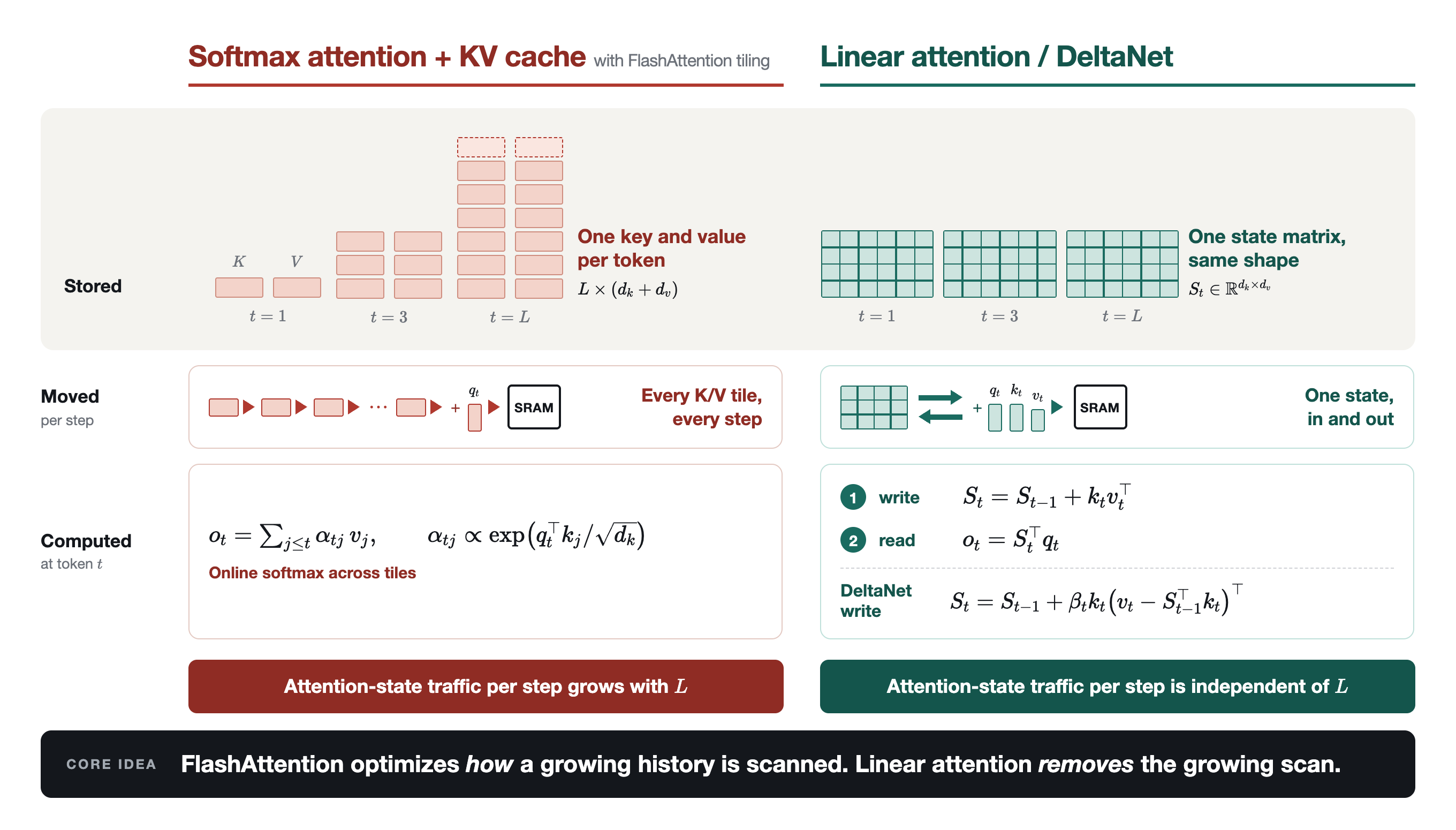
Autoregressive decoding I/O at one layer and attention head. Softmax attention scans a growing KV history; linear attention and DeltaNet read and update a fixed-size state.
- A KV cache stores the keys and values of previous tokens explicitly, so its memory grows with the context.
- Linear attention uses associativity to focus on the key-value product rather than the full query-key attention matrix.
-
The previous context is compressed into a fixed-size state:
\[S_t=S_{t-1}+k_tv_t^\top.\] -
The state can be interpreted as a regression function mapping keys to values:
\[f_S(k)=S^\top k.\] -
DeltaNet replaces the additive write with an error-correcting update:
\[S_t = S_{t-1} +\beta_tk_t (v_t-S_{t-1}^\top k_t)^\top.\] - The same update can be viewed as removing the value currently associated with $k_t$ and writing a corrected value.
- Chunkwise algorithms make the recurrence more suitable for GPU training.
- Gated DeltaNet adds a separate mechanism for rapidly forgetting the broader state.
References
- Mastering LLM Techniques: Inference Optimization — Shashank Verma and Neal Vaidya, NVIDIA Technical Blog, 2023
- Beyond Softmax: The Future of Attention Mechanisms — Jia-Bin Huang
- Transformers are RNNs: Fast Autoregressive Transformers with Linear Attention — Angelos Katharopoulos, Apoorv Vyas, Nikolaos Pappas, and François Fleuret, ICML 2020
- Linear Transformers Are Secretly Fast Weight Programmers — Imanol Schlag, Kazuki Irie, and Jürgen Schmidhuber, ICML 2021
- Parallelizing Linear Transformers with the Delta Rule over Sequence Length — Songlin Yang, Bailin Wang, Yu Zhang, Yikang Shen, and Yoon Kim, NeurIPS 2024
- Gated Delta Networks: Improving Mamba2 with Delta Rule — Songlin Yang, Jan Kautz, and Ali Hatamizadeh, ICLR 2025
Enjoy Reading This Article?
Here are some more articles you might like to read next: